No project description provided

Project description
VIA
VIA is a single-cell Trajectory Inference method that offers topology construction, pseudotimes, automated terminal state prediction and automated plotting of temporal gene dynamics along lineages. VIA combines lazy-teleporting random walks and Monte-Carlo Markov Chain simulations to overcome common challenges such as 1) accurate terminal state and lineage inference, 2) ability to capture combination of cyclic, disconnected and tree-like structures, 3) scalability in feature and sample space. 4) Generalizability to multi-omic analysis. In addition to transcriptomic data, VIA works on scATAC-seq, flow and imaging cytometry data. Please refer to our paper for more details.
Getting Started
Linux Ubuntu 16.04 and Windows 10 Installation
We recommend setting up a new conda environment
conda create --name ViaEnv python=3.7
pip install pyVIA // tested on linux Ubuntu 16.04 and Windows 10
This usually tries to install hnswlib, produces an error and automatically corrects itself by first installing pybind11 followed by hnswlib. To get a smoother installation, consider installing in the following order after creating a new conda environment:
pip install pybind11
pip install hnswlib
pip install pyVIA
install by cloning repository and running setup.py (ensure dependencies are installed)
git clone https://github.com/ShobiStassen/VIA.git
python3 setup.py install // cd into the directory of the cloned VIA folder containing setup.py and issue this command
MAC installation
The pie-chart cluster-graph plot does not render correctly for MACs for the time-being. All other outputs are as expected.
conda create --name ViaEnv python=3.7
pip install pybind11
conda install -c conda-forge hnswlib
pip install pyVIA
install dependencies separately if needed (linux ubuntu 16.04 and Windows 10)
If the pip install doesn't work, it usually suffices to first install all the requirements (using pip) and subsequently install VIA (also using pip). Note that on Windows if you do not have Visual C++ (required for hnswlib) you can install using this link .
pip install pybind11, hnswlib, python-igraph, leidenalg>=0.7.0, umap-learn, numpy>=1.17, scipy, pandas>=0.25, sklearn, termcolor, pygam, phate, matplotlib,scanpy
pip install pyVIA
Jupyter Notebooks
There are several Jupyter Notebooks with step-by-step code for real and simulated datasets. If you experience issues with opening the notebook from github, then copy the Jupyter Notebook URL and paste it into nb viewer https://nbviewer.jupyter.org/
Examples
Expected runtime will be a few minutes or less. Runtime on a "normal" laptop ~5 minutes for EB and less for smaller data. Data for the Jupyter Notebooks and Examples are available in the Datasets folder (smaller files) and larger datasets here.
1.a Toy Data (multifurcation) Multifurcation Jupyter NB
1.b Toy Data (disconnected) Disconnected Jupyter NB
2.a Human Embryoid Bodies (wrapper function)
2.b Human Embryoid Bodies (Configuring VIA) EB Jupyter NB
3.a General input format and wrapper function
3.b General disconnected trajectories wrapper function
More examples with additional code, outputs and details are available as Jupyter Notebooks
1.a/b Toy data (Multifurcation and Disconnected)
Two examples toy datasets with annotations are generated using DynToy are provided.
To run on Linux:
All examples are shown according to Linux OS, small modifications are required to run on a Windows OS (see below)
import pyVIA.core as via
# ensure the data and label files are in csv format when you download/save them
#multifurcation
#the root is automatically set to root_user = 'M1'
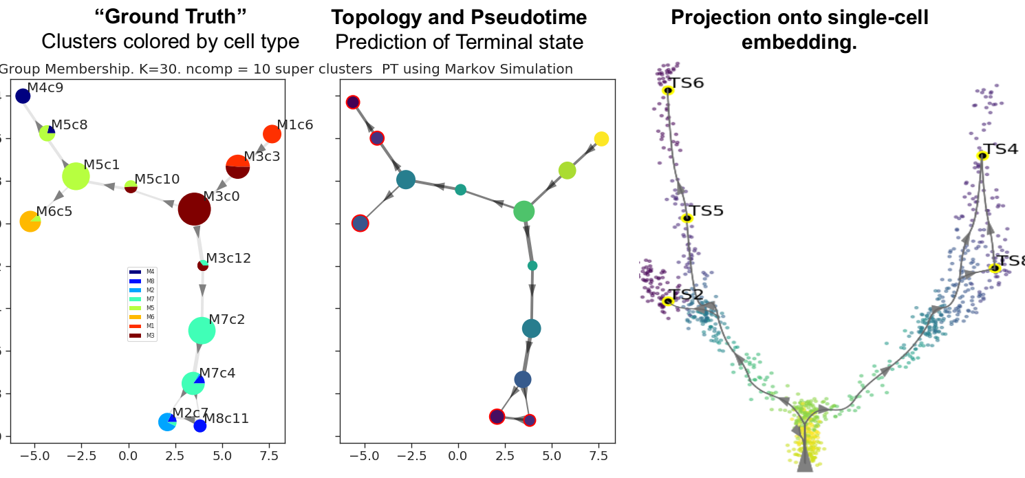
via.main_Toy(ncomps=10, knn=30,dataset='Toy3', random_seed=2,foldername = ".../Trajectory/Datasets/") #multifurcation
#disconnected trajectory
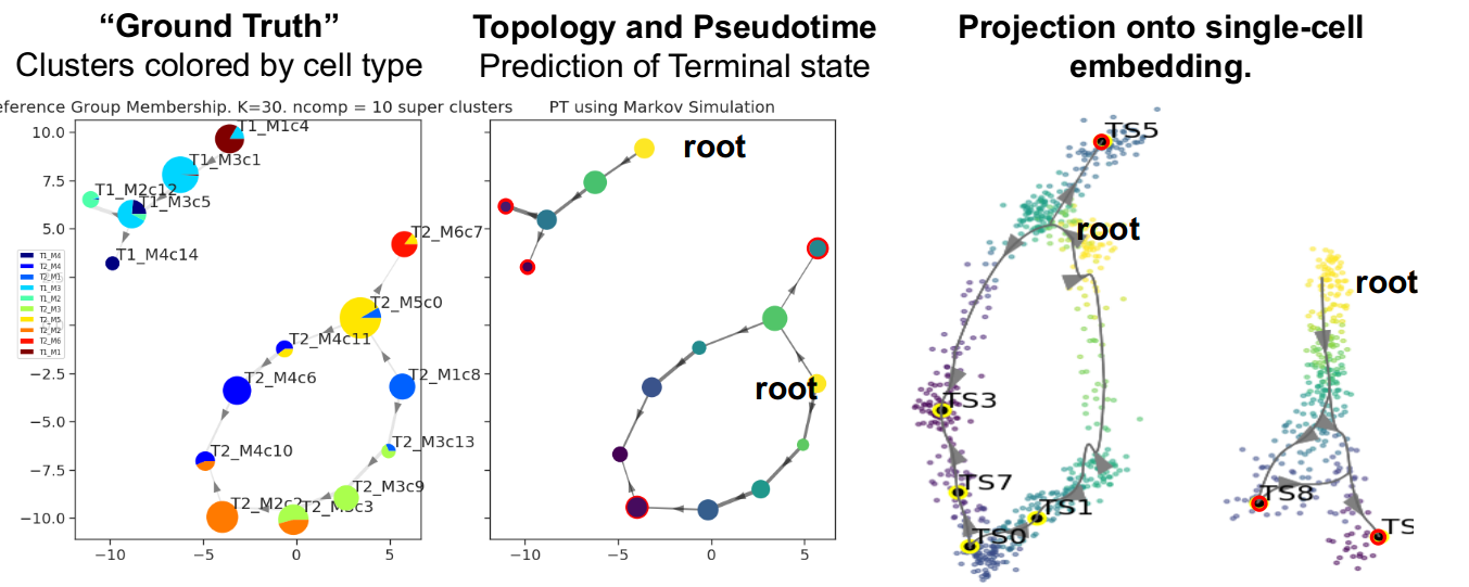
#the root is automatically set as a list root_user = ['T1_M1', 'T2_M1'] # e.g. T2_M3 is a cell belonging to the 3rd Milestone (M3) of the second Trajectory (T2)
via.main_Toy(ncomps=10, knn=30,dataset='Toy4',random_seed=2,foldername =".../Trajectory/Datasets/") #2 disconnected trajectories
Windows (small modifications in calling the code due to the way multiprocessing works in Windows compared to Linux)
To run on Windows:
A few additional lines are required:
#when running from an IDE you need to call the function in the following way to ensure the parallel processing works:
import os
import pyVIA.core as via
f= os.path.join(r'C:\Users\...\Documents'+'\\')
def main():
    via.main_Toy(ncomps=10, knn=30,dataset='Toy3', random_seed=2,foldername= f)
if __name__ =='__main__':
    main()

#when running directly from terminal:
import os
import pyVIA.core as via
f= os.path.join(r'C:\Users\...\Documents'+'\\')
via.main_Toy(ncomps=10, knn=30,dataset='Toy3', random_seed=2,foldername= f)
if __name__ =='__main__':
Output of Multifurcating toy dataset
Output of disconnected toy dataset
2.a Human Embryoid Bodies (wrapper function)
Save the Raw data matrix as 'EBdata.mat'. The cells in this file have been filtered for too small/large libraries by Moon et al. 2019.
Save the phate embedding which is required to run Example 2.a (since the phate operation is
The function main_EB_clean() preprocesses the cells (normalized by library size, sqrt transformation). It then calls VIA to: plot the pseudotimes, terminal states, lineage pathways and gene-clustermap. The visualization method used in this function is PHATE.
#runtime on single core, 8GB RAM 64bit Windows is about 8-10 minutes. This can be lowered by reducing the number of MCMC simulations (num_mcmc_simulations).
import pyVIA.core as via
#Windows example path for folder where EBdata.mat is saved: f= os.path.join(r'C:\Users\...\Documents'+'\\')
via.main_EB_clean(ncomps=30, knn=20, v0_random_seed=24, foldername = f) # Most reasonable parameters of ncomps (10-200) and knn (15-50) work well
2.b Human Embryoid Bodies (Configuring VIA)
If you wish to run the data using UMAP or TSNE (instead of PHATE), or require more control of the parameters/outputs, then use the following code. (See the Jupyter Notebook for detailed output and code). Expected runtime will be around 1-2 minutes using 5 cores, or ~8-10 on "normal" laptop. .
import pyVIA.core as via
#pre-process the data as needed and provide to via as a numpy array
#root_user is the index of the cell corresponding to a suitable start/root cell

v0_too_big = 0.3 #clusters comprising more than 30% of total cell population will be re-clustered by PARC
v1_too_big = 0.05

v0 = via.VIA(input_data, time_labels, jac_std_global=0.15, dist_std_local=1, knn=knn,
             too_big_factor=v0_too_big, root_user=[1], dataset='EB', random_seed=v0_random_seed,
             do_magic_bool=True, is_coarse=True, preserve_disconnected=True)
v0.run_VIA()


tsi_list = get_loc_terminal_states(v0, input_data) #translate the terminal clusters found in v0 to the fine-grained run in v1

v1 = via.VIA(input_data, time_labels, jac_std_global=0.15, dist_std_local=1, knn=knn,
             too_big_factor=v1_too_big, super_cluster_labels=v0.labels, super_node_degree_list=v0.node_degree_list,
             super_terminal_cells=tsi_list, root_user=[1], is_coarse=False, full_neighbor_array=v0.full_neighbor_array,
             full_distance_array=v0.full_distance_array, ig_full_graph=v0.ig_full_graph,
             csr_array_locally_pruned=v0.csr_array_locally_pruned,
             x_lazy=0.95, alpha_teleport=0.99, preserve_disconnected=True, dataset='EB',
             super_terminal_clusters=v0.terminal_clusters, random_seed=21)
v1.run_VIA()

#Plot the true and inferred times and pseudotimes
#Replace Y_phate with UMAP, TSNE embedding
f, (ax1, ax2) = plt.subplots(1, 2, sharey=True)
ax1.scatter(Y_phate[:, 0], Y_phate[:, 1], c=time_labels, s=5, cmap='viridis', alpha=0.5)
ax2.scatter(Y_phate[:, 0], Y_phate[:, 1], c=v1.single_cell_pt_markov, s=5, cmap='viridis', alpha=0.5)
ax1.set_title('Embyroid Data: Days')
ax2.set_title('Embyroid Data: VIA')
plt.show()

#obtain the single-cell locations of the terminal clusters to be used for visualization of trajectories/lineages
super_clus_ds_PCA_loc = via.sc_loc_ofsuperCluster_PCAspace(v0, v1, np.arange(0, len(v1.labels)))
#draw the overall lineage paths on the embedding
via.draw_trajectory_gams(Y_phate, super_clus_ds_PCA_loc, v1.labels, v0.labels, v0.edgelist_maxout,
                         v1.x_lazy, v1.alpha_teleport, v1.single_cell_pt_markov, time_labels, knn=v0.knn,
                         final_super_terminal=v1.revised_super_terminal_clusters,
                         sub_terminal_clusters=v1.terminal_clusters,
                         title_str='Pseudotime and path', ncomp=ncomps)

2D_knn_hnsw = via.make_knn_embeddedspace(Y_phate) #used to visualize the path obtained in the high-dimensional KNN
#draw the individual lineage paths and cell-fate probabilities at single-cell level
via.draw_sc_evolution_trajectory_dijkstra(v1, Y_phate, 2D_knn_hnsw, v0.full_graph_shortpath,
                                      idx=np.arange(0, input_data.shape[0]))
plt.show()
3.a General input format and wrapper function (uses example of pre-B cell differentiation)
Datasets and labels used in this example are provided in Datasets.
# Read the two files:
# 1) the first file contains 200PCs of the Bcell filtered and normalized data for the first 5000 HVG.
# 2)The second file contains raw count data for marker genes

data = pd.read_csv('./Bcell_200PCs.csv')
data_genes = pd.read_csv('./Bcell_markergenes.csv')
data_genes = data_genes.drop(['cell'], axis=1)
true_label = data['time_hour']
data = data.drop(['cell', 'time_hour'], axis=1)
adata = sc.AnnData(data_genes)
adata.obsm['X_pca'] = data.values

# use UMAP or PHate to obtain embedding that is used for single-cell level visualization
embedding = umap.UMAP(random_state=42, n_neighbors=15, init='random').fit_transform(data.values[:, 0:5])

# list marker genes or genes of interest if known in advance. otherwise marker_genes = []
marker_genes = ['Igll1', 'Myc', 'Slc7a5', 'Ldha', 'Foxo1', 'Lig4', 'Sp7']  # irf4 down-up
# call VIA. We identify an early (suitable) start cell root = [42]. Can also set an arbitrary value
via.via_wrapper(adata, true_label, embedding, knn=10, ncomps=20, jac_std_global=0.15, root=[42], dataset='',
            random_seed=1,v0_toobig=0.3, v1_toobig=0.1, marker_genes=marker_genes)
3.b VIA wrapper for generic disconnected trajectory
import scanpy as sc
import pandas as pd

#foldername corresponds to the location where you have saved the Toy Disconnected data (shown in example 2)
#Read in the data and labels
df_counts = pd.read_csv(foldername + "toy_disconnected_M9_n1000d1000.csv", 'rt', delimiter=",")
df_ids = pd.read_csv(foldername + "toy_disconnected_M9_n1000d1000_ids.csv", 'rt', delimiter=",")

# Make AnnData object for wrapper function to read-in data and do PCA
df_ids['cell_id_num'] = [int(s[1::]) for s in df_ids['cell_id']]
df_counts = df_counts.drop('Unnamed: 0', 1)
df_ids = df_ids.sort_values(by=['cell_id_num'])
df_ids = df_ids.reset_index(drop=True)
true_label = df_ids['group_id']
adata_counts = sc.AnnData(df_counts, obs=df_ids)
sc.tl.pca(adata_counts, svd_solver='arpack', n_comps=10)

#Since there are 2 disconnected trajectories, we provide 2 arbitrary roots (start cells).If there are more disconnected paths, then VIA arbitrarily selects roots. #The root can also just be arbitrarily set as [1] and VIA can detect how many additional roots it must add
via.via_wrapper_disconnected(adata_counts, true_label, embedding=adata_counts.obsm['X_pca'][:, 0:2], root=[1,1], preserve_disconnected=True, knn=30, ncomps=10,cluster_graph_pruning_std = 1)

#in the case of connected data (i.e. only 1 graph component. e.g. Toy Data Multifurcating) then the wrapper function from example 3.a can be used:
via.via_wrapper(adata_counts, true_label, embedding=  adata_counts.obsm['X_pca'][:,0:2], root=[1], knn=30, ncomps=10,cluster_graph_pruning_std = 1)
Parameters and Attributes
Parameters
| Input Parameter for class VIA | Description |
|---|---|
data |
(numpy.ndarray) n_samples x n_features. When using via_wrapper(), data is ANNdata object that has a PCA object adata.obsm['X_pca'][:, 0:ncomps] and ncomps is the number of components that will be used. |
true_label |
(list) 'ground truth' annotations or placeholder |
knn |
(optional, default = 30) number of K-Nearest Neighbors for HNSWlib KNN graph |
root_user |
When using one of the example datasets where there is a single root cell type, simply provide the index number of the cell corresponding to a sensible root: root_user = 1. When using the generic via wrapper, this input is in the form of a list containing roots corresponding to index (row number in cell matrix) of root cell. For most trajectories this is of the form [99], for multiple disconnected trajectories an arbitrary list of cells can be provided [1,506,1100] or VIA arbitratily chooses cells. If the root cells of disconnected trajectories are known in advance, then the cells should be annotated with similar syntax to that of Example Dataset in Disconnected Toy Example 1b. |
dist_std_local |
(optional, default = 1) local pruning threshold for PARC clustering stage: the number of standard deviations above the mean minkowski distance between neighbors of a given node. the higher the parameter, the more edges are retained |
jac_std_global |
(optional, default = 0.15) global level graph pruning for PARC clustering stage. This threshold can also be set as the number of standard deviations below the network's mean-jaccard-weighted edges. 0.1-1 provide reasonable pruning. higher value means less pruning. e.g. a value of 0.15 means all edges that are above mean(edgeweight)-0.15*std(edge-weights) are retained. We find both 0.15 and 'median' to yield good results resulting in pruning away ~ 50-60% edges |
too_big_factor |
(optional, default = 0.4) if a cluster exceeds this share of the entire cell population, then the PARC will be run on the large cluster |
x_lazy |
(optional, default = 0.95) 1-x = probability of staying in same node (lazy). Values between 0.9-0.99 are reasonable |
alpha_teleport |
(optional, default = 0.99) 1-alpha is probability of jumping. Values between 0.95-0.99 are reasonable unless prior knowledge of teleportation |
distance |
(optional, default = 'l2' euclidean) 'ip','cosine' |
random_seed |
(optional, default = 42) The random seed to pass to Leiden |
pseudotime_threshold_TS |
(optional, default = 30) Percentile threshold for potential node to qualify as Terminal State |
resolution_parameter |
(optional, default = 1) Uses ModuliartyVP and RBConfigurationVertexPartition |
preserve_disconnected_after_pruning |
(optional, default = False) Cluster-graph pruning can occasionally cause fragmentation that can be repaired (by setting to True) by retaining select edges. |
cluster_graph_pruning_std |
(optional, default =0.15) Usually set to the same value as the PARC clustering level of jac_std_global. To retain more connectivity in the graph underlying the trajectory computations, increase the value |
visual_cluster_graph_pruning |
(optional, default = 0.15) Usually set to the same value as the PARC clustering level of jac_std_global. This does not impact computation of terminal states, pseudotime or lineage likelihoods. It controls the number of edges plotted for visual effect |
num_sim_branch_probability |
(optional), default = 500. Number of MCMCs run per terminal state. This can be safely reduced to 100 when computational resources are limited |
| As shown in the examples, VIA is built to run on a single or double iteration. For extremely large datasets (>1M cells), a single pass is favourable. For mid-size it can be useful to run the double-pass mode which is shown in Example 2b and 3a,b. In the first pass VIA performs a coarser clustering which is useful for capturing terminal states. To increase the resolution of the pseudotime, lineage likelihood and gene trends, we re-run VIA in a second pass which produces a finer cluster-graph and transfers the lineages (terminal states) obtained in the first pass into the second pass. We therefore provide the second pass with the terminal_states obtained in the first pass. To speed up the computation, we also pass the original HNSW KNN graph. The following parameters are used for second passes. |
| Input Parameter | Description |
|---|---|
is_coarse |
(optional, default = True) If running VIA in two steps, for the second fine-grained, set to "False' |
super_cluster_labels |
Set this to v0.labels (clustering output of first pass "v0") |
super_terminal_cells |
super_terminal_cells = via.get_loc_terminal_states(v0, data) |
full_neighbor_array |
full_neighbor_array=v0.full_neighbor_array. KNN graph from first pass of via - neighbor array |
full_distance_array |
full_distance_array=v0.full_distance_array. KNN graph from first pass of via - edge weights |
ig_full_graph |
ig_full_graph=v0.ig_full_graph igraph of the KNN graph from first pass of via |
csr_array_locally_pruned |
csr_array_locally_pruned=v0.csr_array_locally_pruned. CSR matrix of the locally pruned KNN graph |
| Attributes | Description |
|---|---|
labels |
(list) length n_samples of corresponding cluster labels |
edgelist_maxout |
(list) used to draw trajectories on the 2D embedding |
single_cell_pt_markov |
(list) computed pseudotime |
single_cell_bp |
(array) computed single cell branch probabilities (lineage likelihoods). n_cells x n_terminal states. The columns each correspond to a terminal state, in the same order presented in the'terminal_clusters' attribute |
terminal clusters |
(list) terminal clusters found by VIA |
Release history Release notifications | RSS feed


Download files
Download the file for your platform. If you're not sure which to choose, learn more about installing packages.
Source Distribution
Built Distribution
Filter files by name, interpreter, ABI, and platform.
If you're not sure about the file name format, learn more about wheel file names.
Copy a direct link to the current filters
File details
Details for the file pyvia-0.2.4.tar.gz.
File metadata
- Download URL: pyvia-0.2.4.tar.gz
- Upload date:
- Size: 174.6 kB
- Tags: Source
- Uploaded using Trusted Publishing? No
- Uploaded via: twine/5.1.1 CPython/3.10.14
File hashes
| Algorithm | Hash digest | |
|---|---|---|
| SHA256 |
f2bd6360486061bc9a6053c6efda4dfba8fcc39d8d07e39d9b131530b4bf2e39
|
|
| MD5 |
9f3c0115d47f73e29bc27b970890ae9d
|
|
| BLAKE2b-256 |
64232f4d5e9eba3698989a4c538175c068cb695204fc2fd2ce9c8a6bd4c39917
|
File details
Details for the file pyVIA-0.2.4-py3-none-any.whl.
File metadata
- Download URL: pyVIA-0.2.4-py3-none-any.whl
- Upload date:
- Size: 171.8 kB
- Tags: Python 3
- Uploaded using Trusted Publishing? No
- Uploaded via: twine/5.1.1 CPython/3.10.14
File hashes
| Algorithm | Hash digest | |
|---|---|---|
| SHA256 |
001e9f5eef2e0c6b43b4ba43519f22d890221e0d0cde734141cbff59e4076495
|
|
| MD5 |
f1b2464b1bf8823a7758549695d0b7ba
|
|
| BLAKE2b-256 |
fc70cd1d2cdd4f7ef30f9eeadc84dd4c2944747c082f3774bf3d21b22c541e0d
|


