Python utility library for agena.ai to create Bayesian network models from scratch or import existing models and export to agena.ai cloud or local API for calculations.

Project description
Table of Contents
- Description
- Prerequisites and Installation
- Structure of pyagena Classes
- Class and Instance Methods
- Importing a Model from .cmpx
- Creating and Modifying a Model in python
- Agena.ai Cloud with pyagena
- Local agena.ai API with pyagena
- Importing and Exporting Datasets for Batch Calculation
- pyagena Use Case Examples
1. Description
pyagena is a python environment for creating, modifying, and parsing Bayesian network models, and sending the models to agena.ai Cloud or to local agena.ai developer API to execute calculation requests. The environment allows users to read and modify Bayesian networks from .cmpx model files, create new Bayesian networks in python and export to .cmpx and .json files locally, as well as authenticate with agena.ai Cloud or use local agena.ai developer API for model calculations and sensitivity analyses. In the rest of this document, the python environment for agena.ai is referred to as pyagena. pyagena is developed for Python 3.8+.
2. Prerequisites and Installation
You can install pyagena using pip:
pip install pyagena
pyagena requires the following python packages to be installed: requests, pandas, networkx, and matplotlib
In case these were not installed automatically, you can install them with the commands:
pip install requests
pip install pandas
pip install matplotlib
pip install networkx
Once installed, you can import the package in the python script (or a jupyter notebook file) to use. For example:
import pyagena as ag
or
from pyagena import *
3. Structure of pyagena Classes
The Bayesian networks (BNs) in pyagena are represented with several objects: Model, Network, Node, and Dataset. These python objects generally follow their equivalents defined in agena.ai models.
3.1 Model objects
These represent the overall BN. A single .cmpx file corresponds to a singe Model. A BN model can have multiple networks with their own nodes, links between these networks, and datasets.
3.1.1 id
Id of the Model, optional.
3.1.2 networks
A list of all the Network objects in the model. This field will be populated with the create_network() method. See below for more information about Networks.
3.1.3 datasets
A list of all the Dataset objects in the model. When a new Model is created, it will have the default first dataset "Case 1", and it is possible to add new datasets to the model afterwards with the create_dataset() method. See below for more information about Datasets.
3.1.4 network_links
If the Model has multiple networks, it is possible to have links between these networks, following the agena.ai model network_links format.
To see how to create these links, see add_network_link() function later in this document.
3.1.5 settings
Model settings for calculations. It includes the following fields (the values in parantheses are the defaults if settings are not specified for a model):
- discreteTails (False)
- sampleSizeRanked (5)
- convergence (0.01)
- iterations (50)
- tolerance (1)
Model settings can be provided when creating a new model, if not provided the model will come with the default settings. Default settings can be changed later on (with the method change_settings()), or model settings can be reset back to default values (with the method default_settings()). See the correct input parameter format for these functions in the following section. Individual fields in model setting can be adjusted with change_settings() too. Individual setting value can be accessed with syntax model.settings['convergence'].
3.2 Network objects
These represent each network in a BN model. Networks consist of nodes and in a BN model there might be more than one network. These networks can also be linked to each other with the use of input and output nodes. For such links, see Model.network_links field.
The fields that define a Network object are as follows:
3.2.1 id
Id of the Network. Mandatory field to create a new network.
3.2.2 name
Name of the network, optional. If not specified, id of the network is passed onto name field as well.
3.2.3 description
Description, optional. If not specified, the string "New Network" is assigned to description field by default.
3.2.4 nodes
A list of Node objects which are in the network. See below for more information about Nodes.
Note that Network objects do have a create_edge() method but do not have a links field unlike the agena.ai models. As explained in Node.parents section below, this information is stored in Node objects in the python environment. When importing a .cmpx model, the information in links field is used to populate Node.parents fields for each node. Similarly, when exporting to a .cmpx/.json file, the parent-child information in Node.parents field is used to create the links field of the Network field of the .cmpx/.json.
3.3 Node objects
These represent the nodes in a BN. The fields that define a Node object are as follows:
3.3.1 id
Mandatory field to create a new Node object. This is the unique identifier of agena.ai model nodes.
3.3.2 name
Name of the node, optional. If not defined, id of the node will be passed onto the name field too.
3.3.3 description
Description of the node, optional. If not defined, "New Node" will be assigned to the description field.
3.3.4 type
Node type, it can be:
- Boolean
- Labelled
- Ranked
- DiscreteReal
- ContinuousInterval
- IntegerInterval
If it's not specified when creating a new node, the new node is "Boolean" by default if it's not a simulation node; and it is "ContinuousInterval" by default if it's a simulation node.
3.3.5 parents
Other Node objects can be pointed as parents of a Node object. To add parents to a node, see the node method add_parent() or network method create_edge().
Something to keep in mind: the parent-child relationship information is stored at Node level in the python environment thanks to this field, as opposed to the separate links field of a .cmpx/.json file for the agena.ai models. When importing or exporting .cmpx files you do not need to think about this difference, as the file import and export functions handle the correct formats. This difference allows adding and removing Node objects as parents.
3.3.6 simulated
A boolean field to indicate whether the node is a simulation node or not.
3.3.7 distr_type
The table type of the node, it can be:
- Manual
- Expression
- Partitioned
To set the table (distribution) type of a node, see the node method set_distr_type() or the network method set_node_distr_type().
3.3.8 states
States of the node (if not simulated). If states are not specified, depending on the type, sensible default states are assigned. Default states for different node types are:
- "Boolean" or "Labelled" node: "False", "True"
- "Ranked" node: "Low", "Medium", "High"
- "DiscreteReal" node: "0", "1"
- "IntegerInterval" node (if not simulated): "(-Infinity, -1]", "[0, 4]", "[5, Infinity)"
- "ContinuousInterval" node (if not simulated): "(-Infinity, -1)", "[-1, 1)", "[1, Infinity)"
And for a node with the table type (distr_type) "Expression", the default expression is: "Normal(0,1000000)".
To set new states to an existing nodes, see the node method set_states() or the network method set_node_states().
3.3.9 probabilities
If the table type (distr_type) of the node is "Manual", the node will have state probabilities, values in its NPT. This field is a list of lists containing these values. The length of the list depends on the node states and the number of its parents. To see how to set probability values for a node, see the node method set_probabilities() or network method set_node_probabilities().
3.3.10 expressions
If the table type (distr_type) of the node is "Expression" or "Partitioned", the node will have expression(s) instead of the manually defined NPT values.
- If the node's table type is "Expression", the
expressionsfield will be a list with a single expression. - If the node's table type is "Partitioned", the
expressionsfield will be a list of as many expressions as the number of parent node states on which the expression is partitioned.
To see how to set the expressions for a node, see the node method set_expressions() or the network method set_node_expressions().
Possible expressions for the node types are listed below:
Boolean and Labelled:
- Comparative
IntegerInterval
- Binomial
- Exponential
- Geometric
- Hypergeometric
- Negative Binomial
- Normal
- Poisson
- TNormal
- Triangular
- Uniform
ContinuousInterval
- Arithmetic
- Beta
- BetaPert
- ChiSquared
- Exponential
- ExtremeValue
- Gamma
- Logistic
- LogNormal
- Normal
- Student
- TNormal
- Triangle
- Uniform
- Weibull
Ranked
- TNormal
For further information on expressions, please refer to agena.ai modeller manual, Sections 22 (Statistical distributions) and 23 (Expressions).
3.3.11 partitions
If the table type (distr_type) of the node is "Partitioned", in addition to the expressions, the node will have the partitions field. This field is a list of strings, which are ids of the parent nodes on which the node expression is partitioned.
3.3.12 variables
The node variables are called constants on agena.ai Modeller. This field, if specified, sets the constant value for the node observations. For the correct syntax of defining a variable, see set_variable() function.
3.4 Dataset objects
These represent the set of observations in a BN model (cases). A Model can have multiple Dataset objects in its datasets field. When a new Model is created, it always comes with a default Dataset object with the id "Case 1" and with blank observations. It is possible to add more datasets (cases) with their ids. Each Dataset object under a Model can be called a new "case".
3.4.1 id
Id of the dataset (case).
3.4.2 observations
Under each dataset (case), observations for all the observed nodes in all the networks of the model (in terms of their states or values) are listed. If it's hard evidence, observation for a node will have a single value with the weight of 1. If a node in the model has a value in its variable field, this value will be passed onto the dataset (case) with the weight of 1.
3.4.3 results
This field is defined only for when a .cmpx model with calculations is imported or after the model is calculated with the agena.ai Cloud or local API. When creating a new BN in the python environment, this field is not filled in. The results field stores the posterior probability and inference results upon model calculation on agena.ai Cloud or local agena.ai developer API.
4. Class and Instance Methods
The Model, Network, Node, and Dataset objects have their own respective methods to help their definition and manipulate their fields. The python instance methods are used with the . sign following an instance of the class. For example,
example_node.add_parent(example_parent_node)
or
example_network.remove_node(example_node)
or
example_model.create_dataset(example_case)
Before going into the details of methods, a note on displaying success messages and logging info as you go on with the pyagena usage: If you'd like to see the success messages and logging info, you can set the following once at the beginning of the work:
set_verbose(True)
This is for success messages and logging info. The warning and error messages are displayed by default.
To also display timestamps of the messages:
include_timestamps(True)
4.1 Model methods
A Model object consists of networks, network links, datasets, and settings. Once a new Model is created, it is possible to create Networks and Datasets in it. By default, a new Model object comes with a single empty dataset (case) called "Case 1". Following methods can be used to modify Model objects:
4.1.1 create_network(id, name=None, description=None)
A method to create a new Network object in a Model and add it to the networks field of the Model object. The input id is mandatory. The new Network object is added to the Model if the Model does not already have a Network with the given id.
4.1.2 remove_network(id)
A method to remove an existing Network object from the model using its id. Note that removing a Network from a Model doesn't automatically remove its possible network links to other Networks in the model. network-links field of a Model should be adjusted accordingly if needed.
4.1.3 get_network(network_id)
A method to access a Network object in a Model. The Network can be assigned to a variable and used.
4.1.4 add_network_link(source_network_id, source_node_id, target_network_id, target_node_id, link_type, pass_state = optional)
This is the method to add links to a model between its networks. These links start from a "source node" in a network and go to a "target node" in another network. To create the link, the source and target nodes in the networks need to be specified together with the network they belong to (by the Node and Network ids). The input parameters are as follows:
source_network_id=Network.idof the network the source node belongs tosource_node_id=Node.idof the source nodetarget_network_id=Network.idof the network the target node belongs totarget_node_id=Node.idof the target nodelink_type= a string of the link type name. If not specified, it isMarginals. It can be one of the following:- Marginals
- Mean
- Median
- Variance
- StandardDeviation
- LowerPercentile
- UpperPercentile
- State
pass_state= one of theNode.statesof the source node. It has to be specified only if thelink_typeof the link is"State", otherwise is left blank.
Note that links between networks are allowed only when the source and target nodes fit certain criteria. Network links are allowed if:
- Both nodes are the same type and either of them is simulated
- Both nodes are the same type and neither is simulated and both have the same number of states
- Source node is not numeric interval or discrete real and target node is simulated
4.1.5 remove_network_link(source_network_id, source_node_id,target_network_id, target_node_id)
A method to remove network links, given the ids of the source and target nodes (and the networks they belong to).
4.1.6 remove_all_network_links()
A method to remove all existing network links in a model.
4.1.7 create_dataset(dataset_id)
It is possible to add multiple cases to a model. These cases are new Dataset objects added to the datasets field of a model. Initially these cases have no observations and are only defined by their ids. The cases are populated with the enter_observation() function. The create_dataset() function takes the id of the new dataset to be added as input.
4.1.8 remove_dataset(dataset_id)
A method to remove an existing scenario from the model. Input parameter dataset_id is the string which is the id of a dataset (case).
4.1.9 get_dataset(dataset_id)
A method to access a Dataset object in a Model. The Dataset can be assigned to a variable and used.
4.1.10 enter_observation(network_id, node_id, value, dataset_id = optional, variable_input = False)
A method to enter observation to a dataset in the model. Calls the dataset method enter_observation in the background.
To enter the observation to a specific dataset (case), the dataset id must be given as the input parameter dataset. If dataset is left blank, the entered observation will by default go to the first dataset (case) of the model (called "Case 1" by default). This means that if there is no extra datasets created for a model (which by default comes with "Case 1"), any observation entered will be set for this dataset (mimicking the behaviour of entering observation to agena.ai Modeller).
The observation is defined with the mandatory input parameters:
network_id=Network.idof the network the observed node belongs tonode_id=Node.idof the observed nodevalue= this parameter can be:- the value or state of the observation for the observed node (if it is hard evidence)
- the array of multiple values and their weights (if it is soft evidence)
- the value of the observation for a variable of the observed node
dataset_id= optional,Dataset.idof the dataset which will have the observationvariable_input= a boolean parameter, set toTrueif the entered observation is a variable (constant) id for the node instead of an observed value.
A node can have only one observation. This observation can be hard evidence (single state or a single value) or soft evidence (multiple states or multiple values with their weights). If the node has variable(s), the variable value(s) can also be observed. Each variable of the node can have an observation. If the node with variables has observations for its variables and an observation for itself, the variable observations will be ignored and only the node observation will be used in calculations.
4.1.11 remove_observation(network_id, node_id, dataset_id = optional)
A method to remove a specific observation from the model. Calls the dataset method remove_observation in the background. It requires the id of the node which has the observation to be removed and the id of the network the node belongs to.
4.1.12 clear_dataset_observations(dataset_id)
A method to clear all observations in a specific dataset (case) in the model. Calls the dataset method clear_all_observations() in the background.
4.1.13 clear_all_observations()
A method to clear all observations defined in a model. This function removes all observations from all datasets (cases).
4.1.14 change_settings(setting arguments)
A method to change model settings. The input parameters can be some or all of the settings fields. For example:
example_model.change_settings(convergence=0.001, iterations=75)
4.1.15 default_settings()
A method to reset model settings back to default values. The default values for model settings are:
- discreteTails = False
- sampleSizeRanked = 5
- convergence = 0.01
- iterations = 50
- tolerance = 1
4.1.16 save_to_file(filename)
A method to export the Model to a .cmpx or a .json file. This method passes on all the information about the model, its datasets, its networks, their nodes, and model settings to a file in the correct format readable by agena.ai.
Input parameter filename must have a file extension of '.cmpx' or '.json'.
4.1.17 import_data(filename)
A method to import dataset observations to the model using either a .csv or a .json input file. See examples below for the correct format of the input .csv and .json for data import.
4.1.18 export_data(filename, dataset_ids = optional, include_inputs = False, include_outputs = True)
A method to export dataset results or observations from the model to an either .csv or .json output file. See examples below for the format of the output .csv and .json files.
4.1.19 from_cmpx(filepath = "/path/to/model/file.cmpx")
This is the class method to create a Model object from a .cmpx file. The method parses the .cmpx file and creates the python objects based on the model in the file. To see its use, see examples below.
4.1.20 create_csv_template()
This method creates an empty CSV file for the model with the correct format so that it can be filled in and used for import_data(filename). Note that this template includes every single node in the model, not all of which might be observable - you can delete the columns of the nodes which will not be observed. See examples below for its format and use.
4.1.21 create_sensitivity_config(...)
A method to create a sensitivity configuration object if a sensitivity analysis request will be sent to agena.ai Cloud servers or the local API. Its parameters are:
targetNode= target node ID for the analysissensitivityNodes= a list of sensitivity node IDs- (optional)
network= ID of the network to perform analysis on. If missing, the first network in the model is used - (optional)
dataSet= ID of the dataSet (scenario) to use for analysis - (optional)
report_settings= a dictionary for settings for the sensitivity analysis report. The elements of the dictionary are:"summaryStats"(a list with some/all of the following fields)- mean
- median
- variance
- standardDeviation
- upperPercentile
- lowerPercentile
"sumsLowerPercentileValue"(set the reported lower percentile value. Default is 25)"sumsUpperPercentileValue"(set the reported upper percentile value. Default is 75)"sensLowerPercentileValue"(lower percentile value to limit sensitivity node data by. Default is 0)"sensUpperPercentileValue"(upper percentile value to limit sensitivity node data by. Default is 100)
For the use of the function, see Sections 8 and 9.
4.2 Network methods
A Network object is created in a Model object. Once a network of a model is created, the following methods can be used to modify and manipulate the object and its nodes.
4.2.1 create_node(id, name=optional, description=optional, type=optional, simulated=optional, states=optional)
A method to create a new Node object in a Network and add the new node to the nodes field of the Network object. The id of the new node is mandatory whereas name, description, type, simulated, and states are optional arguments. A new Node object is created with the arguments and added to the network if the network does not already have a node with the given id.
4.2.2 remove_node(node_id)
A method to remove an existing Node object from the network. Note that removing a Node from a network doesn't automatically remove it from its previous parent-child relationships in the network. You need to adjust such relationships separately on Node level.
4.2.3 get_node(node_id)
A method to access a Node object in a Network. The Node can be assigned to a variable and used.
4.2.4 create_edge(child_id, parent_id)
A method to add a parent Node to another Node in a Network. It takes node ids as parameters and runs the add_parent() method of a node.
4.2.5 remove_edge(child_id, parent_id)
A method to remove a parent Node from another Node in a Network. It takes node ids as parameters and runs the remove_parent() method of a node.
4.2.6 set_node_probabilities(node_id, new_probs, by_row=False)
A method to modify Nodes in a Network. On the defined Node with the node_id parameter, it calls the node method set_probabilities().
4.2.7 set_node_states
A method to modify Nodes in a Network. On the defined Node with the node_id parameter, it calls the node method set_states().
4.2.8 set_node_expressions
A method to modify Nodes in a Network. On the defined Node with the node_id parameter, it calls the node method set_expressions().
4.2.9 set_node_variable
A method to modify Nodes in a Network. On the defined Node with the node_id parameter, it calls the node method set_variable().
4.2.10 set_node_distr_type
A method to modify Nodes in a Network. On the defined Node with the node_id parameter, it calls the node method set_distr_type().
4.2.11 plot()
A method to plot the graphical structure of a BN network.
4.3 Node methods
Node objects are created in a Network object (see above). Once the nodes of a network are created, it is possible to modify them.
Some Node fields can be modified with a direct access to the field. For example, to update the name or a description information of a Node, simply use:
example_node.name = "new node name"
or
example_node.description = "new node description"
Because changing the name or description of a Node does not cause any compatibility issues. However, some fields such as table type or parents will have implications for other fields. Changing the node parents will change the size of its NPT, changing the node's table type from "Manual" to "Expression" will mean the state probabilities are now defined in a different way. Therefore, to modify such fields of a Node, use the corresponding method described below. These methods will ensure all the sensible adjustments are made when a field of a Node has been changed. To modify the nodes, you can either use the node methods described in this section, or the network methods described in the next section which allow you to modify nodes in the network. Once a network and its nodes are created, it is recommended to use the network methods to modify its nodes.
If you are directly working with Node objects, these are the methods Node objects can call for various purposes with their input parameters shown in parantheses:
4.3.1 set_states(states)
The method to update the states of the Node object. The node states can be defined upon creation if the node is a discrete node. If states are not specified during creation, sensible defaults will be assigned based on the node type. With set_states() it is possible to update node states later on. If the number of new states given with this method is the same as the previous number of node states, state names will be updated. If set_states() changes the number of node states, node probability table size will be adjusted accordingly and probability values will reset to uniform.
4.3.2 add_parent(new_parent)
The method to add a new parent to a node. Equivalent of adding an arc between two nodes on agena.ai Modeller. The input parameter new_parent is another Node object. If new_parent is already a parent for the node, the function does not update the parents field of the node.
When a new parent is added to a node, its NPT values and expressions are reset/resized accordingly.
4.3.3 remove_parent(old_parent)
The method to remove one of the existing parents of a node. Equivalent of removing the arc between two nodes on agena.ai Modeller. The input parameter old_parent is a Node object which has already been added to the parents field of the node.
When an existing parent is removed from a node, its NPT values and expressions are reset/resized accordingly.
4.3.4 set_distr_type(new_distr_type)
A method to set the table type (distr_type) of a node. If a Node is simulated, its table type can be "Expression" or "Partitioned" - the latter is only if the node has discrete parent nodes. If a Node is not simulated, its table type can be "Manual", "Expression", or "Partitioned (if the node has discrete parent nodes)".
Changing the node's distribution type (table type) adjusts its states/probabilities/`expressions`` parameters accordingly.
4.3.5 set_probabilities(new_probs, by_row = False)
The method to set the probability values if the table type (distr_type) of a Node is "Manual". new_probs is a list of lists containing numerical values, and the length of the input list depends on the number of the states of the node and of its parents.
You can format the input list in two different orders. If the parameter by_row is set to True, the method will read the input list to fill in the NPT row by row; if set to False (it is False by default), the method will read the input list to fill in the NPT column by columnn. This behaviour is illustrated with use case examples later in this document.
4.3.6 set_expressions(new_expr, partition_parents = optional)
The method to set the probability values if the table type (distr_type) of a Node is "Expression" or "Partitioned". If the table type is "Expression", new_expr is a list of size one and partition_parents is left untouched. If the table type is "Partitioned", new_expr is a list of expressions for each parent state, and partition_parents is a list of strings for each partitioned parent node's id. See the following sections for examples.
4.3.7 set_variable(variable_name, variable_value)
A method to set variables (constants) for a node. Takes the variable_name and variable_value inputs which define a new variable (constant) for the node.
4.3.8 remove_variable(variable_name)
A method to remove one of the existing variables (constants) from a node, using the variable_name.
4.4 Dataset Methods
The Dataset objects in the models hold the observations and calculation results. The datasets have the following methods.
4.4.1 enter_observation(network_id, node_id, value, variable_name=optional)
A method to enter an observation to a dataset. See Section 4.1.10 for details. Section 4.1.10 is the model method which calls this dataset method after using its parameter dataset_id to determine to which dataset the observation is entered. It is possible to use the dataset method directly to enter observations to the corresponding dataset.
4.4.2 remove_observation(network_id, node_id)
A method to remove an observation from a dataset. See Section 4.1.11 for details. Section 4.1.11 is the model method which calls this dataset method after using its parameter dataset_id to determine from which dataset is the observation is removed.
4.4.3 clear_all_observations()
A method to remove all observations from a dataset. If the model method clear_dataset_observations(dataset_id) is used, it calls this dataset method. Not to be confused with the model method clear_all_observations() which removes all observations from all datasets in the model.
4.4.4 get_result(network_id, node_id)
If the dataset contains calculation results, you can access the results of a specific node in the model with this method.
4.5 agena.ai Cloud Related Functions
pyagena allows users to send their models to agena.ai Cloud servers for calculation. The functions around the server capabilities (including authentication) are described in Section 8.
4.6 agena.ai Local API Related Functions
pyagena allows users to connect to the local agena.ai developer API for calculation. The functions about the local developer API communication are descibed in Section 9.
Local API related functions come with the parameter verbose (set to False by default). If you'd like to see detailed console output, you can call the functions explained in Section 9 with verbose = True. Note that, for this to work, you also need to have enabled global set_verbose(True) setting.
5. Importing a Model from .cmpx
To import an existing agena.ai model (from a .cmpx file), create a new Model object using the from_cmpx() option:
new_model = Model.from_cmpx("/path/to/model/file.cmpx")
This creates a python Model object with all the information taken from the .cmpx file. All fields and sub-fields of the Model object are accessible now. For example, you can see the networks in this model with:
new_model.networks
Each network in the model is a Network object, therefore you can access its fields with the same logic, for example to see the id of the first network and all the nodes in the first network in the BN, use respectively:
new_model.networks[0].id
new_model.networks[0].nodes
Alternatively you can assign the networks to variables with the get method for further use:
net = new_model.get_network(network_id) #assign desired network to a variable
net.nodes #display fields of the selected network
Similarly, each node in a network itself is a Node object. You can display all the fields of a node. Example uses for the second node in the first network of a model:
new_model.networks[0].nodes[0].id
new_model.networks[0].nodes[1].states
Like the networks, you can assign nodes to variables with the get method for further use:
node_one = net.get_node(node_id) #assign desired node to a variable
node_one.states #display fields of the selected node
Once the python model is created from the imported .cmpx file, the Model object as well as all of its Network, Dataset, and Node objects can be manipulated using python methods.
6. Creating and Modifying a Model in python
It is possible to create an agena.ai model entirely in python, without a .cmpx file to begin with. Once all the networks and nodes of a model are created and defined in python, you can export the model to a .cmpx or .json file to be used with agena.ai calculations and inference, locally or on agena.ai Cloud. In this section, creating a model is shown step by step.
6.1 Creating a Model
You can create an empty model and modify its networks and nodes as described below. To create a new model object:
example_model = Model()
which will initiate a new model object with no networks and one default empty dataset (Case 1).
6.2 Creating Networks
You can create network(s) in the model with the create_network() method of a model. For example:
example_net = example_model.create_network(id="example_net")
which will create a new network in the model with no nodes. Note that if you assign the creation method to a variable, the network variable is usable directly in addition to the model now including the new network.
6.3 Creating Nodes
You can create nodes in a network with the create_node() method of a network.
It is recommended to assign the network in a model to a new variable for the ease of future operations. If not assigned upon creation, you can use get_network(), for example:
example_net = example_model.get_network("example_net")
Now we can use the variable net to create and modify nodes in it:
node_one = net.create_node(id="node_one")
Similar no network creation, you can assign the newly created node to its own variable at the time of creation.
If the optional fields are not specified, the nodes will be created with the defaults. The default values for the fields, if they are not specified, are:
- name = node.id
- description = "New Node"
- simulated = False
- type =
- if simulated: "ContinuousInterval"
- if not simulated: "Boolean"
- states =
- if Boolean or Labelled: ["False", "True"]
- if Ranked: ["Low", "Medium", "High"]
- if DiscreteReal: ["0.0", "1.0"]
Once a new node is created, depending on the type and number of states, other fields are given sensible default values too. These fields are distr_type (table type), probabilities or expressions. To specify values in these fields, you need to use the relevant set functions (described above and explained later). The default values for these fields are:
- distr_type =
- if simulated: "Expression"
- if not simulated: "Manual"
- probabilities =
- if distr_type is Manual: discrete uniform distribution, each state has the probability of (1/number of states)
- expressions =
- if distr_type is Expression: "Normal(0,1000000)"
Look at the following new node creation examples:
net.create_node(id = "node_one")
net.create_node(id = "node_two", name = "Second Node")
net.create_node(id = "node_three", type = "Ranked")
net.create_node(id = "node_four", type = "Ranked", states = ["Very low", "Low", "Medium", "High", "Very high"])
Looking up some example values in the fields that define these nodes:
- node_one.id = "node_one"
- node_one.name = "node_one"
- node_one.description = "New Node"
- node_one.type = "Boolean"
- node_one.states = ["False", "True"]
- node_two.id = "node_two"
- node_two.name = "Second Node"
- node_three.type = "Ranked"
- node_three.states = ["Low", "Medium", "High"]
- node_four.states = ["Very low", "Low", "Medium", "High", "Very high"]
- node_one.distr_type = "Manual"
- node_one.probabilities = [[0.5, 0.5]]
- node_three.probabilities = [[0.3333, 0.3333, 0.3333]]
- node_four.probabilities = [[0.2, 0.2, 0.2, 0.2, 0.2]]
Note that probabilities will be a list (of size one) of lists even when there is no parent node.
6.4 Modifying Nodes
To modify nodes they can either be obtained with the network method get_node() and assigned to a new variable, or preferably the network methods which allow the node modification can be used. For the former, as an example:
node_one = net.get_node("node_one")
and now you can use the variable node_one to modify the node in the network.
To update node information, some fields can be simply overwritten with direct access to the field if it does not affect other fields. These fields are node name and description. For example:
node_one.description = "first node we have created"
Other fields can be specified with the relevant set functions. For these, the node methods can directly be used, or preferably the network methods which allow the node modification can be used. When working on a network, it is recommended to use the network methods to modify its nodes, but below both alternatives are shown with examples.
To update the node states, you can use set_states() on a node:
node_one.set_states(["Negative","Positive"])
or set_node_states() on a network:
net.set_node_states("node_one", states = ["Negative", "Positive"])
Note that the input parameter for set_states() or set_node_states() is a list of node names. If this method changes the number of node states, the NPT will be adjusted accordingly and state probabilities will reset to uniform.
To set probability values for a node with a manual table (distr_type), you can use set_probabilities() on a node:
node_one.set_probabilities([[0.2,0.8]])
or set_node_probabilities() on a network:
net.set_node_probabilities("node_one", probabilities = [[0.2,0.8]])
Note that the set_probabilities() or set_node_probabilities() take a list of lists as input, even when the node has no parents and its NPT has only one row of probabilities. If the node has parents, the NPT will have multiple rows which should be in the input list.
Assume that node_one and node_two are the parents of node_three (how to add parent nodes is illustrated later in this section). Now assume that you want node_three to have the following NPT:
| node_one | Negative | Positive | ||
| node_two | False | True | False | True |
| Low | 0.1 | 0.2 | 0.3 | 0.4 |
| Medium | 0.4 | 0.45 | 0.6 | 0.55 |
| High | 0.5 | 0.35 | 0.1 | 0.05 |
There are two ways to order the values in this table for the set_probabilities() method, using the boolean by_row parameter (which is set to False by default). If you want to enter the values following the rows in agena.ai Modeller NPT rather than ordering them by the combination of parent states (columns), you can use by_row = True where each element of the list is a row of the agena.ai Modeller NPT:
net.set_node_probabilities("node_three", probabilities = [[0.1, 0.2, 0.3, 0.4], [0.4, 0.45, 0.6, 0.55], [0.5, 0.35, 0.1, 0.05]], by_row = True)
If, instead, you want to define the NPT with the probabilities that add up to 1 (conditioned on the each possible combination of parent states), you can set by_row = False as the following example:
net.set_node_probabilities("node_three", probabilities = [[0.1, 0.4, 0.5], [0.2, 0.45, 0.35], [0.3, 0.6, 0.1], [0.4, 0.55, 0.05]], by_row = False)
Similarly, you can use the node method set_expressions() or the network method set_node_expressions() to define and update expressions for the nodes without Manual NPT tables. If the node has no parents, you can add a single expression:
net.set_node_expressions("example_node", expressions = ["TNormal(4,1,-10,10)"])
or
example_node.set_expressions(["TNormal(4,1,-10,10)"])
If the node has parents and the expression is partitioned on the parents:
net.set_node_expressions("example_node", expressions = ["Normal(90,10)", "Normal(110,15)", "Normal(120,30)"], partition_parents = ["parent_node_id"])
In the former example the expression is a list of size one, and in the latter the expression is a list with three elements and the second parameter (partition_parameters) is a list which contains the ids of the parent nodes. In the second example, expression input has three elements based on the number of states of the parent node(s) on which the expression is partitioned.
6.5 Creating/Removing Edges in a Network (Adding and Removing Parent Nodes)
When working with a network with nodes in it, you can add edges between nodes with create_edge:
net.create_edge(child_id="node_three", parent_id="node_one")
This method calls the node method add_parent() to add the parent node information to the child node. To do this directly with nodes, you can alternatively use:
node_three.add_parent(node_one)
This adds node_one to the parents list of node_three, and resizes the NPT of node_three (and resets the values to a discrete uniform distribution).
To remove an already existing edge (parent-child relation) in the network, you can use:
net.remove_edge(child_id="node_three", parent_id="node_one")
This method calls the node method remove_parent() on the child node. To use it directly:
node_three.remove_parent(node_one)
This removes node_one from the parents list of node_three, and resizes the NPT of node_three (and resets the values to a discrete uniform distribution).
Below we follow the steps from creation of node_three to the parent modifications and see how the NPT of node_three changes after each step.
- Creating node_tree with only type specified:
net.create_node(id = "node_three", type = "Ranked")
node_three = net.get_node("node_three")
node_three.parents:
[]
node_three.probabilities:
[[0.3333333333333333, 0.3333333333333333, 0.3333333333333333]]

#discrete uniform with three states (default of Ranked node)
- Changing the probabilities:
node_three.set_probabilities([[0.7, 0.2, 0.1]])
node_three.probabilities:
[[0.7, 0.2, 0.1]]
- Adding a parent:
node_three.add_parent(node_one)

#or net.create_edge("node_three", "node_one")
node_three.parents:
[Node: node_one (Boolean)]

# node_one has been added to the parents list of node_three
node_three.probabilities:
[[0.3333333333333333, 0.3333333333333333, 0.3333333333333333],
 [0.3333333333333333, 0.3333333333333333, 0.3333333333333333]]

#  NPT of node_three has been resized based on the number of parent node_one states
# NPT values for node_three are reset to discrete uniform
- Adding another parent:
node_three.add_parent(node_two)

# or net.create_edge("node_three", "node_two")
node_three.parents:
[Node: node_one (Boolean), Node: node_two (Boolean)]

# node_two has been added to the parents list of node_three
node_three.probabilities:
[[0.3333333333333333, 0.3333333333333333, 0.3333333333333333],
 [0.3333333333333333, 0.3333333333333333, 0.3333333333333333],
 [0.3333333333333333, 0.3333333333333333, 0.3333333333333333],
 [0.3333333333333333, 0.3333333333333333, 0.3333333333333333]]

#  NPT of node_three has been resized based on the number of parent node_one and node_two states
# NPT values for node_three are reset to discrete uniform
6.6 Modifying the Model
So far we initially created an "empty" model and populated it with a network and its nodes. It is possible to add multiple networks to the model:
example_model.create_network(id="network_one")
example_model.create_network(id="network_two")
It is also possible to modify a model object regarding its network_links, datasets, and settings.
Network links between networks of the model can be added with the add_network_link() method. For example:
example_model.add_network_link(source_network_id = "network_one", source_node_id = "node_three", target_network_id = "network_two", target_node_id = "node_three", link_type = "Marginals")
For link_type options and allowed network link rules, see add_network_link() in the previous section.
You can remove an existing network link with remove_network_link() method:
example_model.remove_network_link(source_network_id = "network_one", source_node_id = "node_three", target_network_id = "network_two", target_node_id = "node_three")
or you can remove all existing network links in a model with
example_model.remove_all_network_links()
When a new model is created, it comes with a single dataset (case) by default. See next section to see how to add observations to this dataset (case) or add new datasets (cases).
6.7 Creating Datasets (Cases) and Entering Observation
To enter observations to a Model (which by default has one single case), use the enter_observation() function. You need to specify the node (and the network it belongs to) and give the value (one of the states if it's a discrete node, a sensible numerical value if it's a continuous node):
example_model.enter_observation(network_id = network_one, node_id = node_three, value = "High")
Note that this function did not specify any dataset (case). If this is the case, observation is always entered to the first (default) case.
You may choose to add more datasets (cases) to the model with the create_dataset() function:
case_two = example_model.create_dataset("Case 2")
Once added, you can enter observation to the new dataset (case) if you specify the dataset_id parameter in the enter_observation() function:
example_model.enter_observation(dataset_id = "Case 2", network_id = network_one, node_id = node_three, value = "Medium")
6.8 Exporting a Model to .cmpx or .json
Once a python model is defined fully and it is ready for calculations, you can export it to a .cmpx or a .json file:
example_model.save_to_file("example_model.cmpx")
or
example_model.save_to_file("example_model.json")
7. agena.ai Cloud with pyagena
Once the Bayesian network model is prepared and modified and is ready for calculations, you can connect to either agena.ai Cloud or a local agena.ai developer API environment for calculations.
pyagena allows you to authenticate with agena.ai Cloud (using your existing account) and send your model files to Cloud for calculations. The connection between your local python environment and agena.ai Cloud servers uses the python package requests.
7.1 Authentication
The cloud operations use a python object called login to authenticate the user account, and allows user to run further calculations.
To create an account, visit https://portal.agena.ai. Once created, you can use your credentials in pyagena to access the servers.
example_user = login()
If you give no parameters, you will be prompted to enter your username and password for authentication. Alternatively you can pass them as parameters to login constructor:
example_user = login(username, password)
This will send a POST request to authentication server, and will create a logged in user instance (including access and refresh tokens) which will be used to authenticate further operations.
You can choose to see either basic operation result messages or detailed debugging messages when you use the model calculation and sensitivity analysis functions after authentication. You can set the debug message option for the logged in cloud user with:
example_user.set_debug(True)
You can also choose to change the root of the API server URL for operations for the logged in user instance. The default for this is "https://api.agena.ai". To change this, for example:
example_user.set_server_url("http://localhost:8080")
If you'd like to reset the server URL to the default, you can run:
example_user.reset_server_url()
7.2 Model Calculation
Using the login instance created, you can do further operations such as calculations and sensitivity analysis.
calculate() function is used to send a python model object to agena.ai Cloud servers for calculation. This is a method of the logged in user instance. The function takes the following parameters:
modelis the python Model object- (optional)
dataset_idis the id of the dataset that contains the set of observations (.idof one of the.datasetsobjects) if any. If the model has only one dataset (case) with observations, dataset needs not be specified (it is also possible to send a model without any observations).
Currently servers accept a single dataset (a single set of observations) for each calculation, if the python model has multiple datasets (cases), you need to specify which dataset is to be used.
For example,
example_user.calculate(example_model)
or
example_user.calculate(example_model, dataset_id)
If the calculation is successful, this function will update the python model (the relevant .results field in the model's .dataset) with results of the calculation obtained from agena.ai Cloud.
The model calculation computation supports asynchronous request (polling) if the computation job takes longer than 10 seconds. The python client will periodically recheck the servers and obtain the results once the computation is finished (or timed out, whichever comes first).
If you would like to see the calculation results in a .csv format, you can use the Model method export_data() to generate the output file. See Section 9 for examples.
7.3 Sensitivity Analysis
Sensitivity analysis is another cloud server operation for the logged in user instance. For the sensitivity analysis, first you need to crate a sensivity configuration object, using the .create_sensitivity_config(...) method of a Model. For example,
example_sens_config = example_model.create_sensitivity_config(
                      targetNode = "node_one",
                      sensitivityNodes = ["node_two","node_three"],
                      report_settings = {"summaryStats" : ["mean", "variance"]},
                      dataSet = "dataset_id",
                      network = "network_one")
Here, targetNode and sensitivityNodes parameters are mandatory for a sensitivity configuration and the rest is optional with sensible defaults assigned on the cloud servers.
Using the defined configuration object, now you can use the sensitivity_analysis() method of the logged in user instance to send the request to the server. For example,
sa_results = example_user.sensitivity_analysis(example_model, example_sens_config)
If successful, this will return a dict with some information about the process and the results. Unlike calculate(), this method is advised to assign to a variable for future analysis and use. The returned dict includes the following fields:
- lastUpdated
- version
- log
- uuid
- debug
- duration
- messages
- results
- memory
The results contains raw results data for all analysis report options defined, such as tables, tornado graphs, and curve graphs. To access the results:
sa_results.results
You can see the cloud API documentation for further information on the sensitivity analysis response here (Manual/Tools: Sensitivity Analysis/Response).
The sensitivity analysis computation supports asynchronous request (polling) if the computation job takes longer than 10 seconds. The python client will periodically recheck the servers and obtain the results once the computation is finished (or timed out, whichever comes first).
8. Local agena.ai API with pyagena
Agena.ai has a Java based API to be used with agena.ai developer license. If you have the developer license, you can use the local API for calculations in addition to agena.ai modeller or cloud. The local API has Java and maven dependencies, which you can see on its github page in full detail. pyagena allows communications with the local agena developer API.
Local API functions, except for local_api_clone, come with the optional parameter verbose, which is by default set to False. If you choose to display full maven output as a result of the functions, you can set verbose = True in the function calls. You also need to enable verbose logging for the library e.g.:
from pyagena import *
set_verbose(verbose=True)
local_api_compile(verbose=True)
8.1 Prerequisites
For the local API functions to work, the following tools must be available console or terminal:
- git
- Java JDK LTS release (such as 8, 11, 17)
- Maven version 3.6.3 or newer
8.2 Setting up the local API directory
To manually set up the local agena developer API, follow the instructions on the github page for the API: https://github.com/AgenaRisk/api.
Or, for the API setup you can use the python environment:
local_api_clone()
to clone the git repository of the API in your working directory.
Once the API is cloned, you can compile maven environment with:
local_api_compile()
Note that for this to work you need to stay in your current working directory, you don't need to navigate into the cloned api folder. The python function will compile the api directory as long as it's a sub-directory of the current working directory (default behaviour if local_api_clone() is used to clone the repository.)
And if needed, activate your agena.ai developer license with
local_api_activate_license("1234-ABCD-5678-EFGH")
passing on your developer license key as the input parameter.
If you need to deactivate your license,
local_api_deactivate_license()
And if you would like to see the license information:
local_api_show_license()
!! Note that when there is a new version of the agena developer API, you need to re-run local_api_compile() function to update the local repository. Remember that this is done in the working directory which contains the /api/ folder, not in the /api/ folder !!
8.3 Model calculation with the local API
Once the local API is compiled and developer license is activated, you can use the local API directly with your models defined in python. To use the local API for calculations of a model created in python:
local_api_calculate(model, dataset_ids=optional, cache_path=optional)
where the parameter model is a python Model object, dataset_ids is a list of the dataset ids in the Model that you want to calculate, and cache_path is an optional parameter for when you want to use cache for batch case calculations (see below). If no dataset_ids is specified, the calculation will be completed for all existing datasets in the model. Even in the case where one dataset is desired to be calculated, the parameter is a list (of size one).
For example,
local_api_calculate(model = example_model,
                    dataset_ids = ["example_dataset_id"])
This function will temporarily create the .cmpx file for the model and the separate .json file required for the dataset, and send them to the local API (cloned and compiled within the working directory), obtain the calculation result values and update the python Model object with the calculation results.
To calculate multiple datasets in the same model:
local_api_calculate(model = example_model,
                    dataset_ids = ["case_one", "case_two"])
or to calculate all the datasets in the model, simply:
local_api_calculate(model = exmple_model)
Local API calculation also supports the use of a cached result file. This option is useful when you want to be able to resume an interrupted batch calculation, as every dataset will be written to file as soon as it is calculated. This requires an existing output json file to be specified in the cache_path parameter, if calculation results for certain datasets already are in this file, they will not be recalculated, and the datasets given in dataset_ids without results in the existing output file will be calculated.
To use a cached output file:
local_api_calculate(model = example_model,
                    dataset_ids = ["case_three", "case_four"],
                    cache_path = "C:/path/to/file/model_output.json")
If you would like to see the calculation results in a .csv format, you can use the Model method export_data() to generate the output file as described in Section 9.
8.4 Sensitivity Analysis with the local API
You can also run a sensitivity analysis in the local API, using
local_api_sensitivity_analysis(model, sens_config)
Here the sens_config is created by the use of .create_sensitivity_config(...) method of a Model. For example:
example_sens_config = example_model.create_sensitivity_config(
                      targetNode = "node_one",
                      sensitivityNodes = ["node_two","node_three"],
                      report_settings = {"summaryStats" : ["mean", "variance"]},
                      dataSet = "dataset_id",
                      network = "network_one")
Note that, unlike local_api_calculate(), this function does not update the existing Model object but returns a new dict of results. So it's a good practice to assign the function to a variable for future analysis and use.
sa_results = local_api_sensitivity_analysis(model = example_model,
                      sens_config = example_sens_config)
This function will temporarily create the .cmpx file for the model and the separate .json files required for the dataset and sensitivity analysis configuration file, and send them to the local API (cloned and compiled within the working directory), obtain the sensitivity analysis result values and create the results dict. The returned dict includes the result values for displays such as sensitivity tables, tornado graphs, and curves. local_api_sensitivity_analysis() looks at the dataSet field of sens_config to determine which dataset to use, if the field doesn't exist, the default behaviour is to create a new dataset without any observations for the sensitivity analysis.
9 Importing and Exporting Datasets for Batch Calculation
It is possible to use pyagena for batch import/export of data and to use the local agena.ai API for batch operations.
9.1 Importing Data
Section 8.2 already explained that you can calculate multiple datasets at once with the local API. The python model can have multiple datasets created in pyagena or parsed from an input .cmpx model with the datasets. Additionally, for an existing python model, you can use import_data(filename) to import multiple datasets and observations in batch from an input file. The input file can be either a .csv or a .json.
9.1.1 From a .csv File
If the input file is a .csv, it should consist of columns representing the nodes in the networks of the model and each row in the file is a new dataset.
In this file, each row of the data is a single case (dataset) with a set of observed values for nodes in the model. First column of the CSV file is the dataset (case) ids which will be used to create a new dataset for each data row. All other columns are possible evidence variables whose headers follow the "network_id.node_id" format. Thus, each column represents a node in the BN and is defined by the node id and the id of the network to which it belongs. The column header for the first one (dataset names) can be anything, 'Case' is the header name when create_csv_template() is used.
An example CSV format is as below:
| Case | network_one.node_one | network_one.node_two | network_one.cont_node | network_two.node_one | network_two.node_two |
|---|---|---|---|---|---|
| Case 1 | Negative | True | 20 | Negative | False |
| Case 2 | Positive |
True | Negative | True | |
| New Case | Positive | False | 18 | Positive |
Once the model is defined in pyagena and the .csv file with the observations is prepared, you can use import_data(filename) to generate scenarios for the BN:
example_model.import_data(filename="./example_data.csv")
This will look up all the rows in the .csv file and create new datasets (cases) in the model for each row whose id does not already exist in the model datasets. If the row id already is the id of an existing dataset, the existing dataset will be updated with the information in the input file. Once the model has a dataset for each row of the input file, all the values of the nodes will be entered as observations to their datasets.
Missing values must be blank cells in the dataset. If there are missing values in the dataset, it will not fill in any observation for that specific node in that specific dataset (case).
You can use create_csv_template() function on a Model object to create an empty .csv file with the correct format for all the nodes and networks in the model. You can then delete the columns for the nodes that are not observed.
9.1.2 From a .json File
The method import_data(filename) also accepts .json file inputs. In this case the .json file should have a list of datasets to be added to the model in the correct format regarding the field names and values. For example:
[{
    "id": "dataset_one",
    "observations": [
      {
        "network": "net_one",
        "node": "node_one",
        "entries" : [
          {
            "weight": 1,
            "value": "Low"
          }
      ]
      },
      {
        "network": "net_one",
        "node": "node_two",
        "entries" : [
          {
            "weight": 1,
            "value": 5.0
          }
      ]}]}]
The input file can be used with the import method:
example_model.import_data(filename="./example_data.json")
This will look up the ids of all the datasets in the .json input, create new datasets in the model for those whose id does not already exist in the model. If the id of any dataset in the input file already exists in the model, that dataset will be updated with the information from the input file. The observations for all the datasets will be imported to the model. If the .json file contains results for any dataset, the results are imported too.
9.2 Exporting Data to a .csv File
It is also possible to export model data to either a .csv or a .json file. The method export_data(...) allows the export of (calculated) results as well as observations in the datasets.
9.2.1 To a .csv File
If the output of the export_data(...) is a .csv file, it can either export observations (inputs) or the results (outputs) of a model dataset.
To export calculation results of all the datasets in a model to a .csv file:
example_model.export_data(filename="./example_output.csv", include_inputs=False, include_outputs=True)
This will generate a .csv file with the following format:
| Case | Network | Node | State | Probability |
|---|---|---|---|---|
| Case 1 | Network 1 | Node 1 | State 1 | 0.2 |
| Case 1 | Network 1 | Node 1 | State 2 | 0.3 |
| Case 1 | Network 1 | Node 1 | State 3 | 0.5 |
| Case 1 | Network 1 | Node 2 | State 1 | 0.3 |
| Case 1 | Network 1 | Node 2 | State 2 | 0.7 |
| Case 1 | Network 1 | Node 3 | State 1 | 0.1 |
| Case 1 | Network 1 | Node 3 | State 2 | 0.8 |
| Case 1 | Network 1 | Node 3 | State 3 | 0.1 |
You can see the posterior probabilities for all the nodes calculated in the model. If you choose to export certain datasets, you can specify:
example_model.export_data(filename="./example_output.csv", dataset_ids = ["Case 1", "Case 2"], include_inputs=False, include_outputs=True)
If you choose to export only observations (inputs) and not the state probabilities of the calculated nodes:
example_model.export_data(filename="./example_output.csv", include_inputs=True, include_outputs=False)
Let's assume the Case 1 has the following three observations:
- Node 1: observed State 2
- Node 2: observed State 1
- Node 3: soft evidence p(State 2)=0.5, p(State 3)=0.5
The export method will generate a .csv with the following format:
| Case | Network | Node | State | Probability |
|---|---|---|---|---|
| Case 1 | Network 1 | Node 1 | State 2 | 1 |
| Case 1 | Network 1 | Node 2 | State 1 | 1 |
| Case 1 | Network 1 | Node 3 | State 2 | 0.5 |
| Case 1 | Network 1 | Node 3 | State 3 | 0.5 |
If you're planning to use Microsoft Excel to display and work with the generated .csv file, it is recommended to set the parameter excel_compatibility to True in the export_data() function. This makes sure the state names are displayed correctly as text in the Excel environment: if for some nodes in the networks the state name includes a "-" before or between values (for example, "-Infinity - 7.0" or "40.0 - 45.0"), some spreadsheet apps like MS Excel misinterpret this as a formula instead of text, excel_compatible = True sends the state names in quotes for MS Excel to interpret as text (this behaviour might add extra characters to state names if the resulting csv is opened with other spreadsheet/text editing apps, in that case setting the excel_compatibility = False, which is the default behaviour, is required).
9.2.2 To a .json File
If the export output is a .json file, then it will contain a list of datasets with all their fields (id, observations, results). .json output can have either inputs, outputs, or both at the same time.
For example,
example_model.export_data(filename="./example_output.json", include_inputs=True, include_outputs=True)
will list all the datasets in the model in the exported .json file such as:
[{
    "id": "dataset_one",
    "observations": [
      {
        "network": "net_one",
        "node": "node_one",
        "entries" : [
          {
            "weight": 1,
            "value": "Low"
          }
      ]
      },
      {
        "network": "net_one",
        "node": "node_two",
        "entries" : [
          {
            "weight": 1,
            "value": 5.0
          }
      ]}],
    "results": [
      {
        "network": "net_one",
        "node": "node_four",
        "resultValues": [
          {
            "label": "Low",
            "value": 0.2
          },
          {
            "label": "High",
            "value": 0.8
          }
        ],
        "summaryStatistics": {
          "confidenceInterval": 50,
          "entropy": 0,
          "percentile": 0.5,
        }
      }]}]
If inputs are not included, observations field is blank. If outputs are not included, results field is blank.
10. pyagena Use Case Examples
In this section, some use case examples of pyagena environment are shown.
10.1 Asia BN Model
This is a BN which calculates the risk of certain medical conditions such as tuberculosis, lung cancer, and bronchitis from two casual factors - smoking and whether the patient has been to Asia recently. Additionally two other pieces of evidence are available: whether the patient is suffering from dyspnoea (shortness of breath) and whether a positive or negative X-ray test result is available.
We can start with creating the model:
asia = Model()
Now create a network in this model (and assign it to a variable for ease of further operations):
asia.create_network(id="asia_net")
net = asia.get_network("asia_net")
Now we can add the nodes to the network:
net.create_node(id="A", name="Visit to Asia?")
net.create_node(id="S", name="Smoker?")

net.create_node(id="T", name="Has tuberculosis")
net.create_node(id="L", name="Has lung cancer")
net.create_node(id="B", name="Has bronchitis")

net.create_node(id="TBoC", name="Tuberculosis or cancer")

net.create_node(id="X", name="Positive X-ray?")
net.create_node(id="D", name="Dyspnoea?")
All the nodes are binary so we do not need to specify the type or states. Then we can add the edges to the network between nodes (adding relevant nodes as parents to the child nodes):
net.create_edge(child_id="T", parent_id="A")
net.create_edge(child_id="L", parent_id="S")
net.create_edge(child_id="B", parent_id="S")
net.create_edge(child_id="TBoC", parent_id="T")
net.create_edge(child_id="TBoC", parent_id="L")
net.create_edge(child_id="X", parent_id="TBoC")
net.create_edge(child_id="D", parent_id="TBoC")
net.create_edge(child_id="D", parent_id="B")
At the moment all nodes have default uniform NPTs, we can define the NPT values:
net.set_node_probabilities(node_id="A", new_probs=[[0.99, 0.01]])
net.set_node_probabilities(node_id="T", new_probs=[[0.99, 0.01],[0.95, 0.05]])
net.set_node_probabilities(node_id="L", new_probs=[[0.9, 0.1], [0.99, 0.01]])
net.set_node_probabilities(node_id="B", new_probs=[[0.7, 0.3], [0.4, 0.6]])
net.set_node_probabilities(node_id="TBoC", new_probs=[[1, 0], [0, 1], [0, 1], [0, 1]])
net.set_node_probabilities(node_id="X", new_probs=[[0.95, 0.05], [0.02, 0.98]])
net.set_node_probabilities(node_id="D", new_probs=[[0.9, 0.1], [0.2, 0.8], [0.3, 0.7], [0.1, 0.9]])
Now we can choose to use the model in any possible way: exporting to a .cmpx file for agena.ai modeller, sending it to agena.ai cloud, or sending it to the local agena.ai developer API for calculations. For example:
asia.save_to_file("asia_bn.json")
10.2 Diet Experiment Model
This is a BN which uses experiment observations to estimate the parameters of a distribution. In the model structure, there are nodes for the parameters which are the underlying parameters for all the experiments and the observed values inform us about the values for these parameters. The model in agena.ai Modeller is given below:
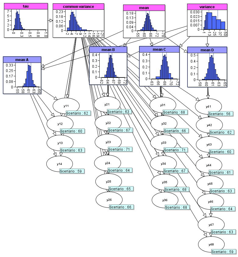
In this section we will create this model entirely in pyagena. We can start with creating an empty model and create the network in it:
diet = Model()

diet.create_network("Hierarchical_Normal_Model_1")
net = diet.get_network("Hierarchical_Normal_Model_1")
Now we can add nodes to the network. Let's start with mean and variance nodes:
#Creating mean and variance nodes

net.create_node(id="mean", simulated=True)
net.set_node_expressions(node_id="mean", expressions=["Normal(0.0,100000.0)"])

net.create_node(id="variance", simulated=True)
net.set_node_expressions(node_id="variance", expressions=["Uniform(0.0,50.0)"])
Common variance and tau nodes:
#Now we create the "common variance" and its "tau" parameter nodes

net.create_node(id="tau", simulated=True)
net.set_node_expressions(node_id="tau", expressions=["Gamma(0.001,1000.0)"])

net.create_node(id="common_var", name="common variance", simulated=True)
net.create_edge(child_id="common_var", parent_id="tau")
net.set_node_expressions(node_id="common_var", expressions=["Arithmetic(1.0/tau)"])
Now we can create the four mean nodes, using a for loop and list of Nodes:
#Creating a list of four mean nodes, "mean A", "mean B", "mean C", and "mean D"

mean_names = ["A", "B", "C", "D"]
means_list = []

for mn in mean_names:
    this_id = "mean" + mn
    this_name = "mean " + mn
    net.create_node(id=this_id, name=this_name)
    net.create_edge(child_id=this_id, parent_id="mean")
    net.create_edge(child_id=this_id, parent_id="variance")
    net.set_node_expressions(node_id=this_id, expressions=["Normal(mean,variance)"])
    means_list.append(this_id)
Now we can create the experiment nodes, based on the number of observations which will be entered:
# Defining the list of observations for the experiment nodes
# and creating the experiment nodes y11, y12, ..., y47, y48

observations = [[62, 60, 63, 59],
                [63, 67, 71, 64, 65, 66],
                [68, 66, 71, 67, 68, 68],
                [56, 62, 60, 61, 63, 64, 63, 59]]

for i, (obs, mn) in enumerate(zip(observations, means_list)):
    for j, ob in enumerate(obs):
        this_id = "y"+str(i)+str(j)
        net.create_node(id=this_id, simulated=True)
        net.create_edge(child_id=this_id, parent_id="common_var")
        net.create_edge(child_id=this_id, parent_id=mn)
        net.set_node_expressions(node_id=this_id, expressions=["Normal("+mn+",common_var)"])
We enter all the observation values to the nodes:
# Entering all the observations

for i, obs in enumerate(observations):
    for j, ob in enumerate(obs):
        this_node_id = "y" + str(i) + str(j)
        diet.enter_observation(network_id=net.id,
        node_id=this_node_id,
        value=ob)
Now the model is ready with all the information, we can export it to either a .json or a .cmpx file for agena.ai Modeller calculations, send it to agena.ai Cloud or to local agena.ai developer API.
# To create a local .cmpx file
diet_model.save_to_file("./diet_model_example.cmpx")

# Or sending it to local agena.ai developer API for calculation
local_api_calculate(diet_model, "Case 1")

# Or sending it to agena.ai Cloud for calculation
user = login()
user.calculate(diet_model, "Case 1")


Download files
Download the file for your platform. If you're not sure which to choose, learn more about installing packages.
Source Distribution
Built Distribution
Filter files by name, interpreter, ABI, and platform.
If you're not sure about the file name format, learn more about wheel file names.
Copy a direct link to the current filters
File details
Details for the file pyagena-1.0.4.tar.gz.
File metadata
- Download URL: pyagena-1.0.4.tar.gz
- Upload date:
- Size: 82.3 kB
- Tags: Source
- Uploaded using Trusted Publishing? No
- Uploaded via: twine/5.1.1 CPython/3.8.0
File hashes
| Algorithm | Hash digest | |
|---|---|---|
| SHA256 |
6638e2fe0d3247c54b9c34320458ddf8ae0a634b6c4955072300fe065dc955d1
|
|
| MD5 |
044483c7633c602769dedca963075816
|
|
| BLAKE2b-256 |
f3c34e093227df155021712e475c43a95f7af8dcae33415f9bf442a5b0897591
|
File details
Details for the file pyagena-1.0.4-py3-none-any.whl.
File metadata
- Download URL: pyagena-1.0.4-py3-none-any.whl
- Upload date:
- Size: 51.0 kB
- Tags: Python 3
- Uploaded using Trusted Publishing? No
- Uploaded via: twine/5.1.1 CPython/3.8.0
File hashes
| Algorithm | Hash digest | |
|---|---|---|
| SHA256 |
a999b3fd830101ae6ec276d35b0c9c9a84619e47eaf35a8dcea639df8a3f0ec5
|
|
| MD5 |
0dea4aaa5888dd0d893de1d25b0193bd
|
|
| BLAKE2b-256 |
7457f9354a0b02d058834ef422813c631d63ce9606433bed8c585f3aad1ba990
|


