
PyAtoms
Simulates scanning probe microscopy (SPM) images. Please read our preprint describing PyAtoms: https://arxiv.org/abs/2412.18332.
(Formerly named: SPM Simulator, Atom Simulator)

Dependencies:
- Python 3.10 or newer
- NumPy
- Matplotlib
- SciPy
- QtPy
- PyQt5 or PyQt6
PyAtoms is compatible with both PyQt5 and PyQt6 through QtPy. PyQt6 is installed by default when PyAtoms is installed using pip.
Installation instructions - macOS and WIndows
Install with pip
PyAtoms can be installed using pip:
pip install pyatoms-spm
After installation, launch PyAtoms by typing:
pyatoms
Run from source
PyAtoms can also be run directly from the source code.
-
Click the green Code button at the top of this GitHub page and select Download ZIP.
-
Extract the downloaded ZIP file.
-
Open a terminal or command line:
- Windows: open Command Prompt, PowerShell, or the Anaconda Prompt.
- macOS: open the Terminal application.
-
In the terminal, navigate to the extracted PyAtoms folder.
If the ZIP was extracted into your Downloads folder, you can usually use:
Windows Command Prompt:
cd %USERPROFILE%\Downloads\PyAtoms-main
Wndows PowerShell:
cd "$HOME\Downloads\PyAtoms-main"
macOS:
cd ~/Downloads/PyAtoms-main
If you extracted the folder somewhere else, replace the path above with the location of your extracted PyAtoms folder.
-
Install the required Python packages.
For PyQt6:
python -m pip install numpy scipy matplotlib QtPy PyQt6
Or, if you use PyQt5:
python -m pip install numpy scipy matplotlib QtPy PyQt5
-
From inside the extracted PyAtoms folder, start PyAtoms with:
python -m pyatoms.PyAtoms_GUI
PyAtoms is compatile with both PyQt5 and PyQt6 through QtPy.
Known issues
02-Sep-2026: Pyatoms is compatile with both PyQt5 and PyQt6 through QtPy. PyQt6 is installed by default when installing PyAtoms through pip.
06-Nov-2025: PyAtoms is currently not compatible with PyQt 6. Still compatible with latest PyQt5 (5.15.11)
28-Oct-2024: No known issues. Works correctly with latest version of Matplotlib (3.9.2)
For windows users:
- Make sure python is installed and that its path is set in your environment
- To check if it is, open the command line and type
python -V - Alternatively, if you installed python, NumPy, SciPy, etc. through Anaconda for Windows, you can run the above code through the Anaconda prompt.
For any other issues or crash reports, suggestions, contact gutierrez@physics.ucla.edu
How to use
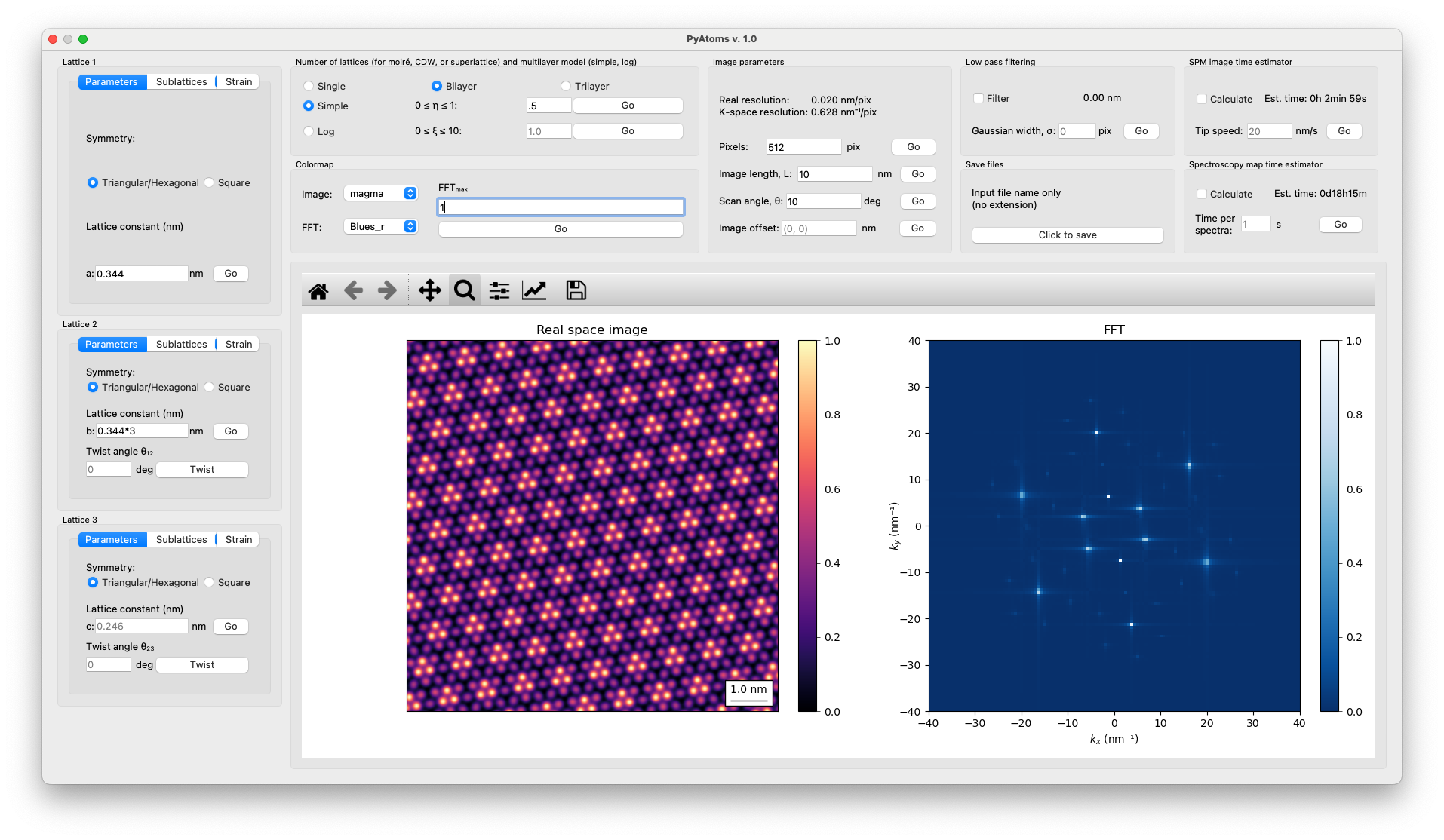
Note that all fields accept typical mathematical operations in python and NumPy such as + - * / sqrt log and all valid NumPy functions func can be called via np.func().
-
Number of lattices (moiré, CDW, superlattice) and Moiré model (Simple, Log)
- Choose to simulate a 1, 2 or 3 layer lattice
- Lattice 1 parameters change the single/first layer.
- Lattice 2 only works if bilayer/trilayer are selected. These change the second lattice.
- Lattice 3 only works if trilayer is selected. These change the third lattice.
- Choose the model to simulate the moiré/CDW/superlattice
Simple: This minimal toy model approximates the moiré image, $T_M$, as the weighted sum between the sum of the individual lattices, $\sum_l Z_l$, and the product of the lattices, $\prod_l Z_l$ and is given by $T_M \propto (1-\eta)\sum_l Z_l + \eta\prod_L Z_l$. This toy model provides a good match to experimental STM images and offers a wide image contrast. However, the Fourier transforms -- by design -- contains only the first order atomic Bragg and moiré lattice peaks. The image is normalized such that $0\leq T_M \leq 1$.eta, $\eta$ : A phenomenological parameter we use to weigh the relative strength of the sum of lattices, $\sum_l Z_l$, to the product of lattices, $\prod_L Z_l$. $\eta$ is a real number between 0 and 1: The moiré/superlattice image for $\eta=0$ purely the sum and $\eta=1$ is purely the product.
Log: This model, described by Joucken et al ( Carbon 83, 48 (2015). ) is rooted in the constant-current tunneling process and takes into account the distance of the multilayers to the STM tip. The moiré/superlattice image, $T_M^L$, is approximated as $T_M^L \propto \ln|Z_1 + Z_2 e^{-\xi}|$ (bilayer) or $T_M^L \propto \ln|Z_1 + Z_2 e^{-\xi} + Z_3 e^{-2\xi}|$ (trilayer). This model provides a good match to both experimental STM images and their Fourier transforms, at the cost of limited image contrast.xi, $\xi$ : The ratio of the inter-layer distance, $d$, and out-of-plane wavefunction decay length, $\lambda$: $\xi = d/\lambda$. $\xi$ is a real number between 0 and 10: For $\xi=0$, the intensity of the lattices is maximized; for $\xi$ = 10, only the top lattice, $Z_1$, is imaged.
- Choose to simulate a 1, 2 or 3 layer lattice
-
Image parameters
Real resolution: Current spatial resolution, defined as L/pix, in units of nm/pix.K-space resolution: Current spatial resolution in reciprocal space, defined as 2π/L, in units of nm⁻¹/pix.Pixels: number of pixels. Must be an integer or a mathematical expression of integers.Image length, L: length of the image window in nanometers. Must be a real number or a mathematical expression of real numbers.Scan angle, θ: Rotation (counter-clockwise) of the atomic lattice. Must be a real number or a mathematical expression of real numbers.Image offset: Location of center of image. Must be a pair of real numbers, or a mathematical expression of real numbers, separated by a comma, e.g. -1.2,4.5.
-
Colormap
Real space image: colormap of the real space simulated atomic lattice.FFT: colormap of the 2D fast Fourier transform.
-
Low pass filtering
Gaussian width, σ: radius of a Gaussian mask in real space in units of pixels. The half-width at half-max of the gaussian is shown as a white circle in the bottom left corner of the image.- The radius of the gaussian mask in nanometers is shown in the text box.
-
Save files
- Click to save the files to a specific directory.
- Clicking will open the file explorer.
- Navigate to the directory you want to save the files in
- Input a
filenameto save as
- It will save a folder called
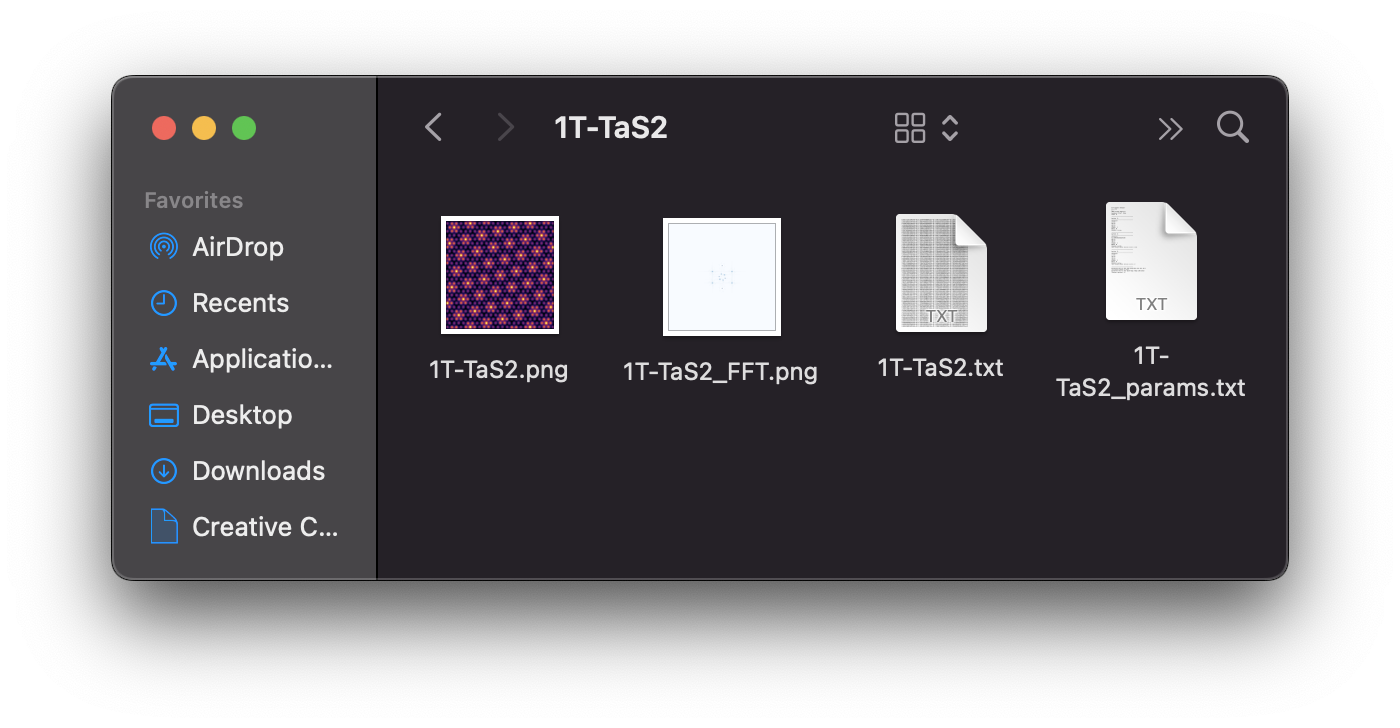
filenamewith 4 files:-
.png images of the real space and FFT, .txt file of the real space image, .txt file of the parameter values
-
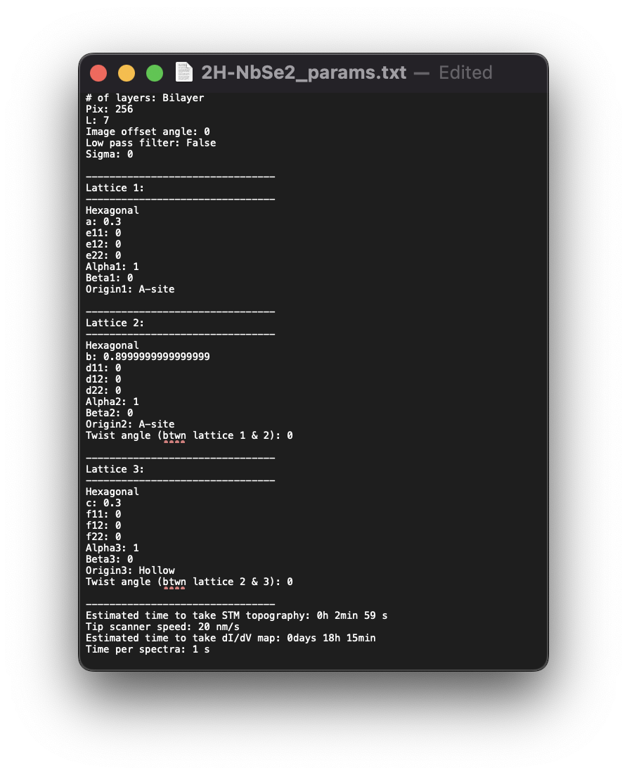
filename.png,filename_FFT.png,filename.txt,filename_params.txt -
Example of folder with saved files:
-
Example of params .txt file:
-
- Click to save the files to a specific directory.
-
SPM image time estimator
Tip velocity: Velocity of the tip, $v_t$ across 1 line in nanometers/second. The total image time is calculated by considering the total pixels, scanning left/right and in a single slow-scan direction (upwards, for example). This time is estimated via $T_{im} = (2 * N_{pix} * L) / v_t$, where $N_{pix}$ is the number of pixels in the image, $L$ is the length of the image in nanometers, and the factor 2 takes into account the left/right fast-scan direction.
-
Spectroscopy map Time estimator
Time per spectra: Total time in seconds (including overhead) to record a single spectrum, $T_{spec}$ i.e. one dI/dV(V) sweep. We assume that spectra are recorded in one direction along both the fast- and slow-scan direction. The time is estimated via $T_{map} = N_{pix}^2 * T_{spec} + (2 * N_{pix} * L) / v_t$.
-
Lattices
-
Parameters tab
symmetry: Choose to simulate either a triangular/hexagonal or square lattice.Lattice constant: periodicity/spacing between atoms in nanometers.Twist angle: twists the second lattice with respect to the first lattice (in Lattice 2 params) // twists the third lattice with respect to the second lattice (in Lattice 3 params)
-
Sublattices tab -- only affects hexagonal (triangular/honeycomb) lattices
-
Lattice site at the image
origin: choose whether theoriginshould be a hollow site, an A-site atom or a B-site atom- To test this, set
L = 1and click the different options for the origin
- To test this, set
-
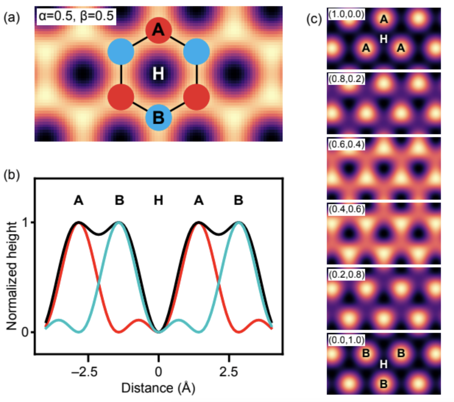
Weight of sublattices:
alpha1, $\alpha_1$ : weight of A sublatticebeta1, $\beta_1$: weight of B sublattice
-
For a triangular lattice:
alpha = 1,beta = 0 -
For a honeycomb lattice:
alpha = 1,beta = 1
-
-
Strain tab
- Apply the 2D strain tensor, $e_{xy}$, where the $x$-axis is defined as the local direction of that lattice, i.e. the strain tensor rotates with the local axes set by
thetaortwist angle. See https://doi.org/10.1103/PhysRevB.80.045401.
- Apply the 2D strain tensor, $e_{xy}$, where the $x$-axis is defined as the local direction of that lattice, i.e. the strain tensor rotates with the local axes set by
-
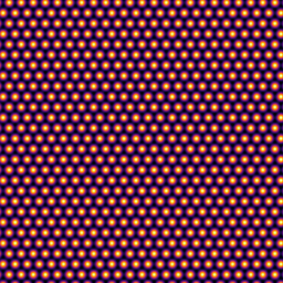
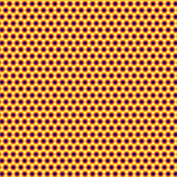
Examples
-
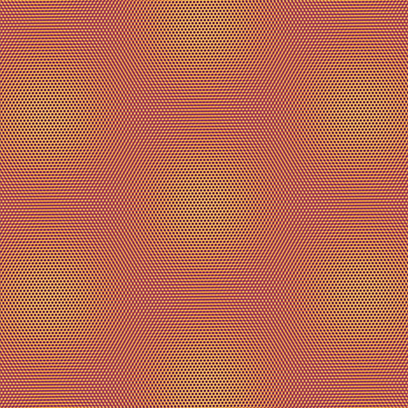
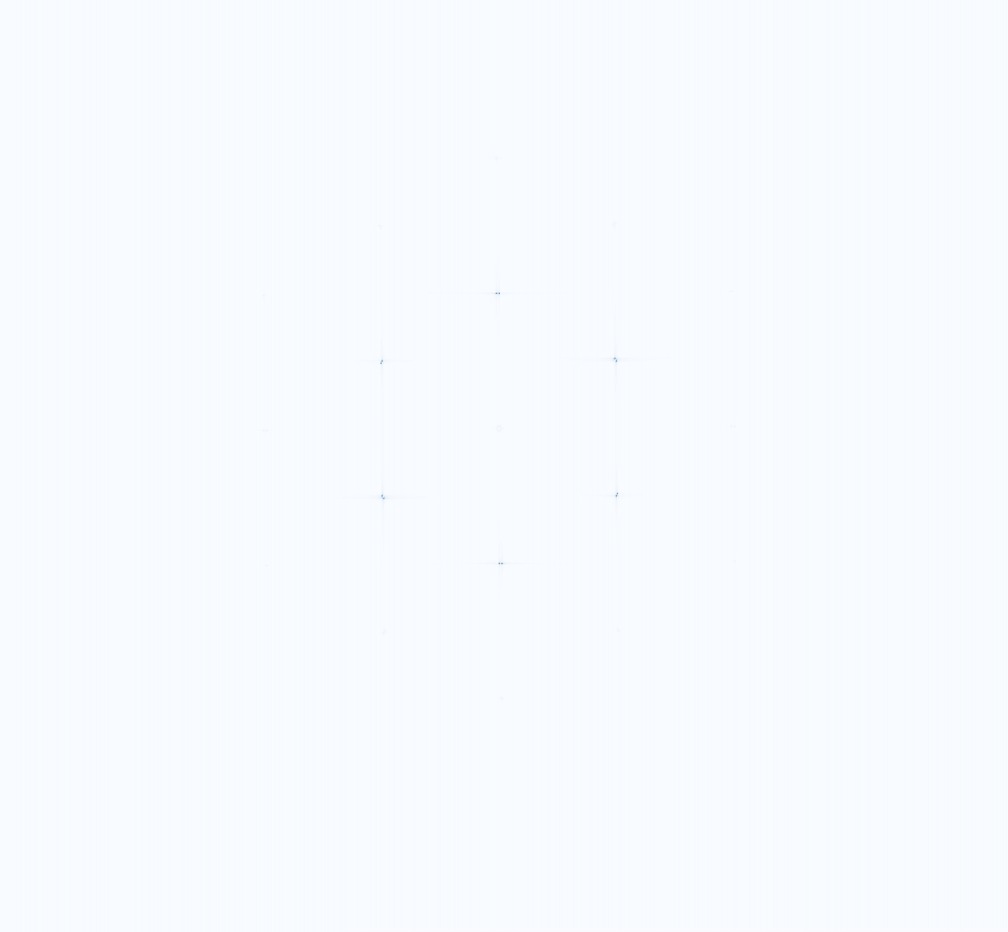
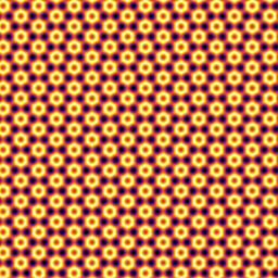
Twisted bilayer graphene with $1.1^\circ$ twist angle.
Moire lattice: bilayerSimpleeta$\eta$ : 0.5L = 35Pixels = 1024- Lattice 1:
- Parameters:
Hexagonal,a = 0.3
- Sublattices:
A-site,alpha1 = 1,beta1 = 1
- Strain:
e11=e12=e22=0
- Parameters:
- Lattice 2:
- Parameters:
Hexagonal,b = 0.3,Twist angle = 1.1
- Sublattices:
A-site,alpha2 = 1,beta2 = 1
- Strain:
d11=d12=d22=0
- Parameters:
-
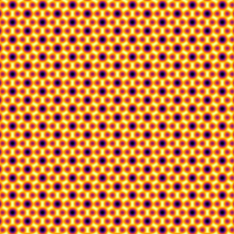
1T-TaS2 with $(\sqrt{13}\times\sqrt{13})R13.9^\circ$ charge density wave superlattice.
Moire lattice: bilayerSimpleeta$\eta$ : 0.5L = 7Pixels = 256Theta = 0- Lattice 1:
- Parameters:
Hexagonal,a = 0.3
- Sublattices:
A-site,alpha1 = 1,beta1 = 0
- Strain:
e11=e12=e22=0
- Parameters:
- Lattice 2:
- Parameters:
Hexagonal,b = 0.3*np.sqrt(13),Twist angle = 13.9
- Sublattices:
A-site,alpha2 = 1,beta2 = 0
- Strain:
d11=d12=d22=0
- Parameters:
-
2H-NbSe2 with $(3\times 3)R0^\circ$ charge density wave superlattice.
Moire lattice: bilayerSimpleeta$\eta$ : 0.5L = 7Pixels = 256Theta = 0- Lattice 1:
- Parameters:
Hexagonal,a = 0.3
- Sublattices:
A-site,alpha1 = 1,beta1 = 0
- Strain:
e11=e12=e22=0
- Parameters:
- Lattice 2:
- Parameters:
Hexagonal,b = 0.3*3,Twist angle = 0
- Sublattices:
A-site,alpha2 = 1,beta2 = 0
- Strain:
d11=d12=d22=0
- Parameters:
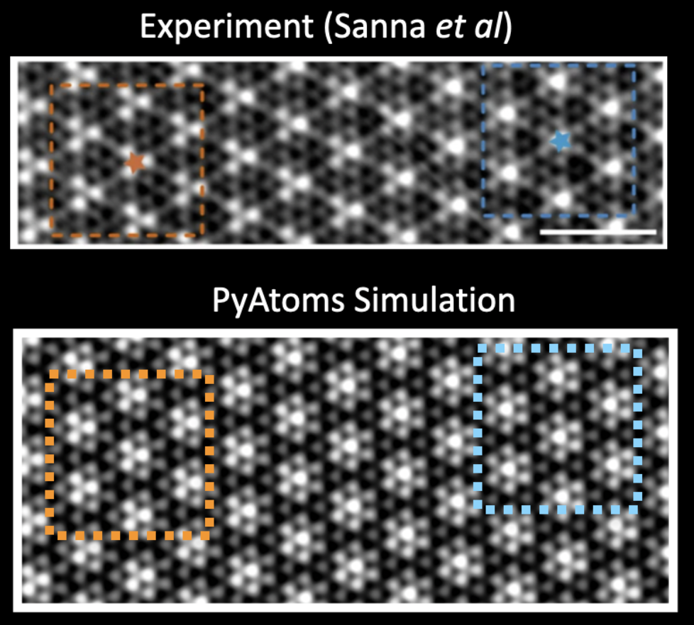
Here is an example where PyAtoms can simulate real data.
Top: Experimental measurement of NbSe2 showing a CDW phase gradient from bond- to site-centered from Sanna et al npj Quantum Materials 7, 6 (2022).
Bottom: PyAtoms simulation of this phase gradient by adding a small discommensuration term, δ, so that the CDW superlattice is given by (3 + δ)x(3 + δ)R0°.
-
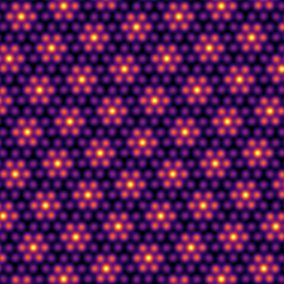
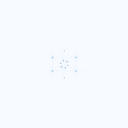
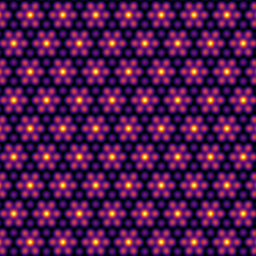
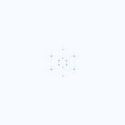
Kekule-O (trivial) distorted graphene with $(\sqrt{3}\times\sqrt{3})R30^\circ$ superlattice.
Moire lattice: bilayerSimpleeta$\eta$ : 0.5L = 7Pixels = 256Theta = 0- Lattice 1:
- Parameters:
Hexagonal,a = 0.3
- Sublattices:
Hollow,alpha1 = 1,beta1 = 1
- Strain:
e11=e12=e22=0
- Parameters:
- Lattice 2:
- Parameters:
Hexagonal,b = 0.3*sqrt(3),Twist angle = 30
- Sublattices:
Hollow,alpha2 = 1,beta2 = 0
- Strain:
d11=d12=d22=0
- Parameters:
-
Kekule-O (topological) distorted graphene with $(\sqrt{3}\times\sqrt{3})R30^\circ$ superlattice.
Moire lattice: bilayerSimpleeta$\eta$ : 0.5L = 7Pixels = 256Theta = 0- Lattice 1:
- Parameters:
Hexagonal,a = 0.3
- Sublattices:
Hollow,alpha1 = 1,beta1 = 1
- Strain:
e11=e12=e22=0
- Parameters:
- Lattice 2:
- Parameters:
Hexagonal,b = 0.3*sqrt(3),Twist angle = 30
- Sublattices:
Hollow,alpha2 = 1,beta2 = 1
- Strain:
d11=d12=d22=0
- Parameters:
1 maintainer

Metadata
1 maintainer
Release files for pyatoms-spm 2.1.0
For a detailed explanation of source distributions (sdists) and built distributions (wheels), please see the package formats documentation.
Source distribution (sdist)
| File | Size | Uploaded | |
|---|---|---|---|
| pyatoms_spm-2.1.0.tar.gz | 792.8 kB | Details |
Built distribution (wheel)
| File | Interpreter | ABI | Platform | Reset |
|---|---|---|---|---|
| pyatoms_spm-2.1.0-py3-none-any.whl | Python 3 | none | any | Details |
Total release size: 1.6 MB
Release files / pyatoms_spm-2.1.0.tar.gz
| Download URL | pyatoms_spm-2.1.0.tar.gz |
|---|---|
| Size | 792.8 kB |
| Tags | Source |
|
SHA-256 checksum How to use checksums |
02ee18610120965efd33ddcd79a7ebb749583acfa33fa2123bac238ebc4b8522
|
|
BLAKE2b-256 checksum How to use checksums |
b6be57042d17a0f75e90c1dc7510c7c10722584d57953a6018a0910515575f18
|
| Upload date | |
|
Uploaded using Trusted Publishing? What is trusted publishing? |
No |
| Uploaded via |
twine/7.0.0 CPython/3.13.5
|
Release files / pyatoms_spm-2.1.0-py3-none-any.whl
| Download URL | pyatoms_spm-2.1.0-py3-none-any.whl |
|---|---|
| Size | 789.3 kB |
| Tags | Python 3 |
|
SHA-256 checksum How to use checksums |
47e283f3cbef8d70f8d8c5c7f016a4b17f43b3db9b7ae6c9ed95250f0abcc049
|
|
BLAKE2b-256 checksum How to use checksums |
5b5789f83a7aa3722e1f919741866ff987ceeaf9dd95068713213994fa1f052b
|
| Upload date | |
|
Uploaded using Trusted Publishing? What is trusted publishing? |
No |
| Uploaded via |
twine/7.0.0 CPython/3.13.5
|














