Bayesian unit-root and cointegration tests for panel data, with publication-quality tables and visualisations.

Project description
pybayescointur
Bayesian unit-root & cointegration tests for panel data
Four published methodologies, one consistent API, publication-quality tables & visualisations.


pybayescointur collects four Bayesian approaches to nonstationarity in
panel data behind a single, friendly interface. Where the classical panel
unit-root / cointegration toolbox relies on asymptotics and point hypotheses,
the Bayesian approach integrates nuisance parameters out, treats the
autoregressive root (and the cointegrating rank) as random, and returns
directly interpretable posterior odds ratios, posterior model
probabilities and Bayes factors.
| # | Method | Function | Reference |
|---|---|---|---|
| 1 | Panel unit root via Posterior Odds Ratio (trend / augmentation) | bayesian_panel_unit_root |
Kumar, Chaturvedi & Afifa (2016) |
| 2 | Panel unit root with structural break in mean & variance (14 PORs) | bayesian_break_unit_root |
Kumar & Agiwal (2019) |
| 3 | Model comparison under cross-sectional dependence (8 models) | bayesian_csd_comparison |
Meligkotsidou, Tzavalis & Vrontos |
| 4 | Panel cointegration (VECM, rank inference) | bayesian_panel_cointegration |
Koop, Leon-Gonzalez & Strachan (2006) |
Table of contents
- Installation
- Quick start
- Method 1 — Panel unit root (Posterior Odds Ratio)
- Method 2 — Structural break in mean & variance
- Method 3 — Cross-sectional dependence
- Method 4 — Panel cointegration
- Tables & visualisation
- Data & simulators
- API reference
- How the numbers are computed
- Citing
- Author
Installation
# from source (recommended while in beta)
git clone https://github.com/merwanroudane/pybayescointur.git
cd pybayescointur
pip install -e ".[all]"        # core + plotly + rich

# minimal core only
pip install -e .
Dependencies: numpy, scipy, pandas, matplotlib (core);
plotly and rich are optional (interactive figures and colourful tables).
Quick start
import pybayescointur as pbc

# --- a near-unit-root, trend-stationary panel (rho = 0.92, n=4, T=80) ---
panel = pbc.simulate_par_panel(n=4, T=80, rho=0.92, seed=1)

res = pbc.bayesian_panel_unit_root(panel, model="augmented", k=2)
print(res)
#  POR  beta_01 : 3.1e-40   ->  Reject H0: series is TREND STATIONARY

pbc.por_table(res)          # pretty, colour-highlighted console table
Every estimator returns a rich result object that
- prints a formatted report (
print(res)), - exports a tidy
DataFrame(res.to_frame()), and - feeds directly into the plotting helpers (
pbc.plot_*).
Method 1 — Panel unit root (Posterior Odds Ratio)
Kumar, J., Chaturvedi, A. & Afifa, U. (2016). Bayesian Unit Root Test for Panel Data. EERI Research Paper 14/2016.
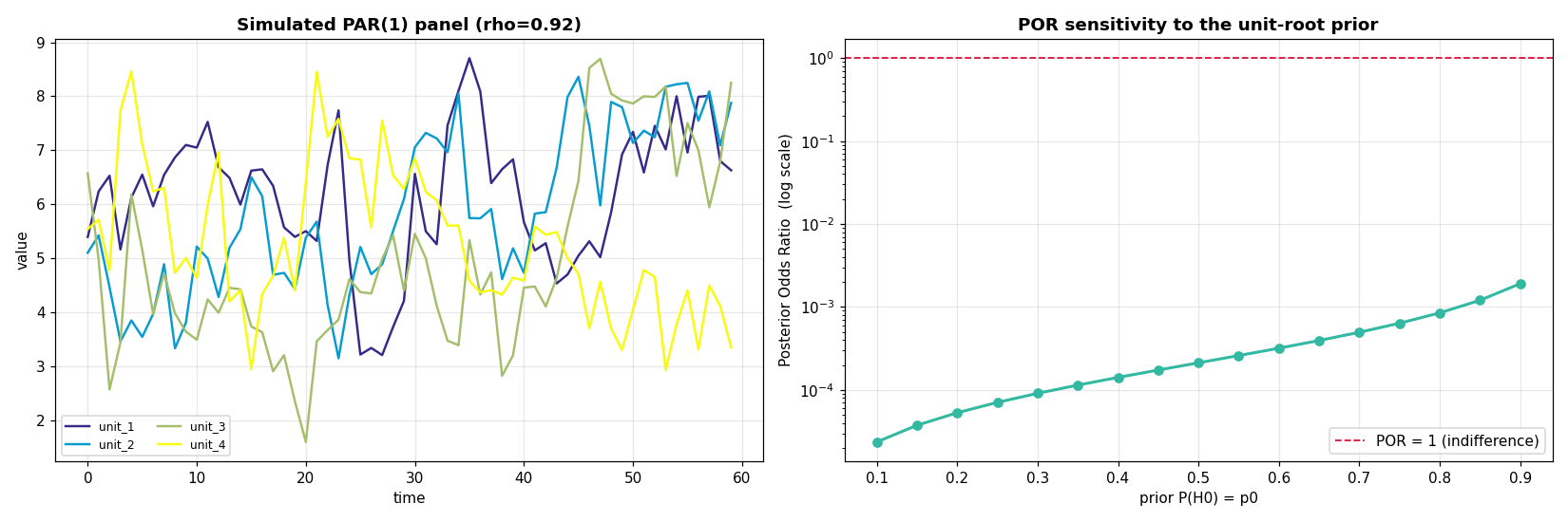
Model. For a panel {y_it ; i = 1..n ; t = 1..T}
y_it = mu_i + delta_i * t + u_it, u_it = rho * u_{i,t-1} + eps_it
The unit-root null H0: rho = 1 (difference stationary) is tested against
H1: a < rho < 1 (trend stationary). The posterior odds ratio beta_01
integrates rho out of the posterior:
beta_01 < 1→ reject the unit root → trend stationarybeta_01 > 1→ fail to reject → difference stationary (unit root)
Two specifications are available: model="trend" (Theorem 1, linear trend)
and model="augmented" (Theorem 2, trend + k lagged differences per unit).
import pybayescointur as pbc

panel = pbc.simulate_par_panel(n=4, T=80, rho=0.92, seed=1)

# linear trend only
r1 = pbc.bayesian_panel_unit_root(panel, model="trend")

# trend + 2 augmentation terms, custom prior P(H0)=0.4, custom lower bound a
r2 = pbc.bayesian_panel_unit_root(
    panel, model="augmented", k=2, p0=0.4, a=-0.5, vartheta=1.0,
)
print(r2)
pbc.por_table(r2)
Bayesian Panel Unit-Root Test  (Posterior Odds Ratio)
Kumar, Chaturvedi & Afifa (2016)
--------------------------------------------------------
  model                 : trend + aug(order 2)
  cross-section units n : 4
  time periods T        : 79
  rho_hat (MLE)         : 0.9123
  POR  beta_01          : 3.07e-40
  Decision: Reject H0 (unit root) -> series is TREND STATIONARY
Note. As the authors themselves emphasise, the trend-only POR is only reliable when the estimated
rho_hatis close to one; otherwise prefer the augmented specification (which is the one used in the paper's application).
Method 2 — Structural break in mean & variance
Kumar, J. & Agiwal, V. (2019). Panel data unit root test with structural break: A Bayesian approach. Hacettepe J. Math. & Stat. 48(4), 1213–1231. doi:10.15672/HJMS.2018.626
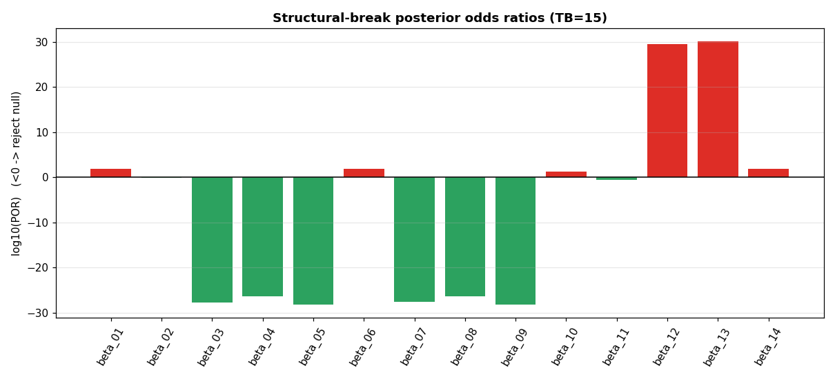
A PAR(1) panel with a single common break at TB, allowing a shift in the
mean (mu_i1 != mu_i2) and in the error variance (lambda != 1). Eight
nested hypotheses (H1–H8) combine rho = 1 vs rho ∈ (a,1) with the
presence/absence of each break; their marginal posterior probabilities give
the fourteen posterior odds ratios POR1 … POR14. beta < 1 favours the
numerator hypothesis.
import pybayescointur as pbc

panel = pbc.simulate_break_panel(
    n=3, T=25, TB=15, rho=0.95, lam=5.0,
    mu1=(30, 40, 50), mu2=(300, 400, 500), seed=0,
)

res = pbc.bayesian_break_unit_root(panel, TB=15)
print(res)
pbc.break_table(res)          # all 14 PORs, colour-coded by decision

# search the break point
for tb in range(8, 21):
    r = pbc.bayesian_break_unit_root(panel, TB=tb)
    print(tb, r.por[4])       # POR4: DS-no-break vs TS-break-both
Method 3 — Cross-sectional dependence
Meligkotsidou, L., Tzavalis, E. & Vrontos, I. D. A Bayesian Analysis of Unit Roots in Panel Data Models with Cross-sectional Dependence.
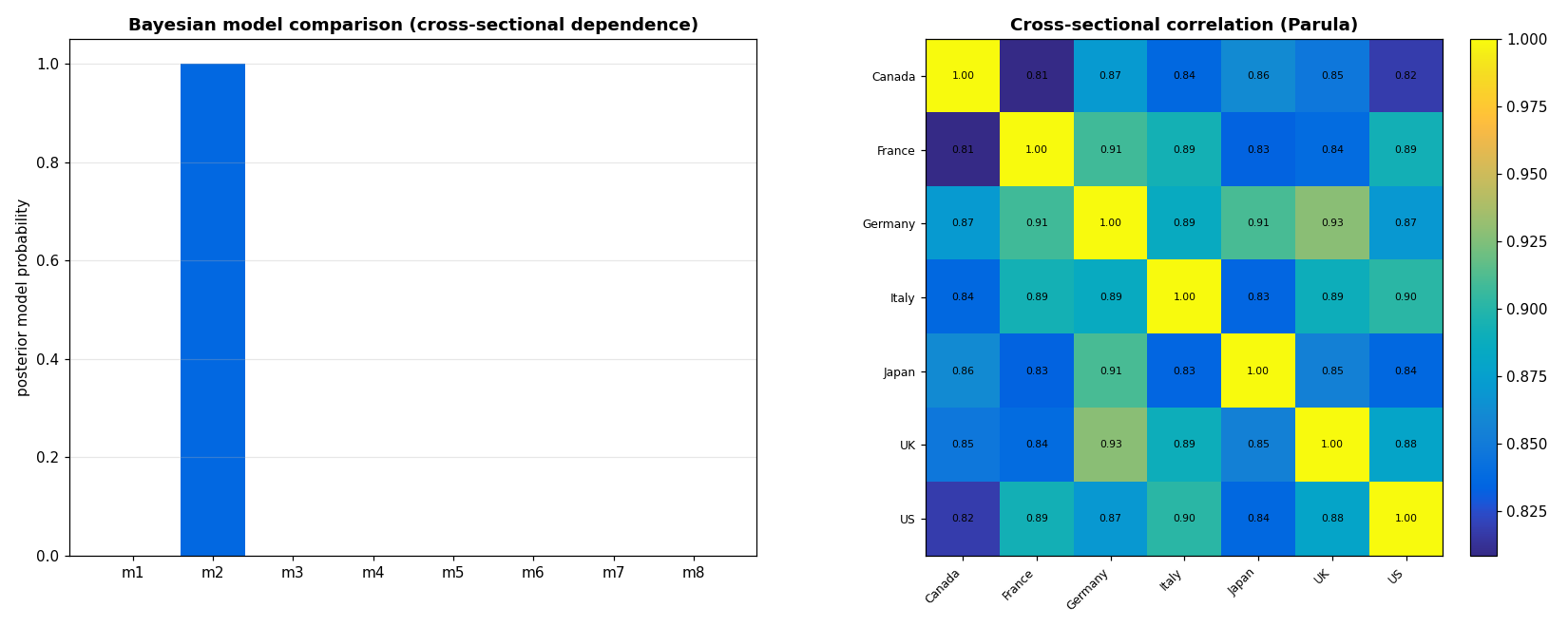
Eight competing models are ranked by their marginal likelihoods / posterior model probabilities:
| model | dynamics | trend | errors |
|---|---|---|---|
| m1 | stationary | no | independent |
| m2 | stationary | no | cross-dependent |
| m3 | stationary | yes | independent |
| m4 | stationary | yes | cross-dependent |
| m5 | random walk | no drift | independent |
| m6 | random walk | no drift | cross-dependent |
| m7 | random walk | drift | independent |
| m8 | random walk | drift | cross-dependent |
import pybayescointur as pbc

gdp = pbc.load_g7_like_gdp()           # synthetic, cross-dependent G7 log-GDP
res = pbc.bayesian_csd_comparison(gdp)

print(res)                             # ranked posterior model probabilities
pbc.csd_table(res)
print(res.correlation_frame().round(2))   # estimated cross-sectional correlations
Bayesian Panel Unit-Root Model Comparison
Meligkotsidou, Tzavalis & Vrontos  (cross-sectional dependence)
------------------------------------------------------------
   m2  P=1.0000  logML=    684.57  stationary, no trend, cross-dependence  <= best
   m4  P=0.0000  logML=    659.94  stationary, trend, cross-dependence
   ...
  Most probable model: m2 (cross-sectional dependence)
The cross-dependent models dominate, and the recovered correlations are high and positive (0.8–0.93) — exactly the empirical pattern reported for the G7.
Method 4 — Panel cointegration
Koop, G., Leon-Gonzalez, R. & Strachan, R. (2006). Bayesian Inference in a Cointegrating Panel Data Model.
Each unit i has its own VECM
Δy_{i,t} = alpha_i beta_i' y_{i,t-1} + Σ_h Gamma_{i,h} Δy_{i,t-h} + Phi_i d_t + eps_{i,t}
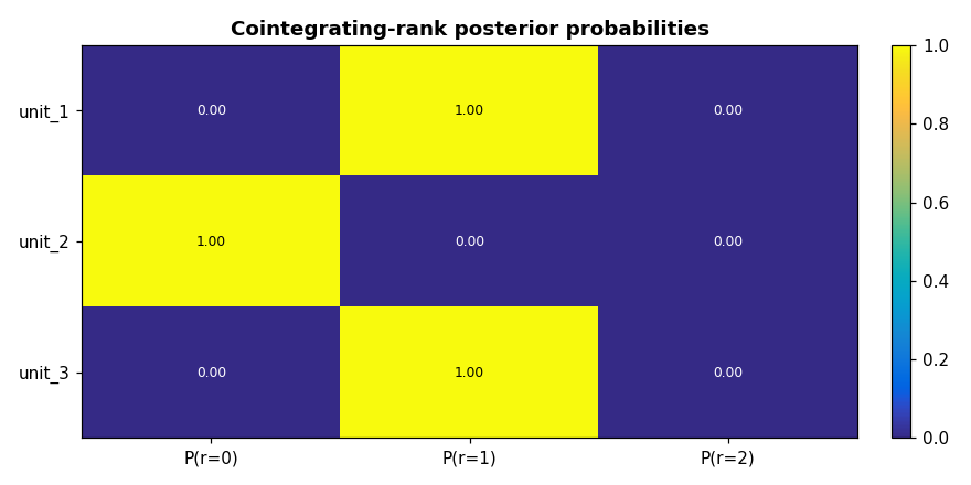
with possibly unit-specific cointegrating rank r_i = rank(alpha_i beta_i').
The rank of each unit is inferred via Savage-Dickey density-ratio Bayes
factors against the no-cointegration model (r_i = 0), and a common-rank
posterior is reported.
import pybayescointur as pbc

# unit 1: rank 1, unit 2: rank 0, unit 3: rank 1
panels = pbc.simulate_vecm_panel(N=3, n=2, T=150, ranks=[1, 0, 1], seed=3)

res = pbc.bayesian_panel_cointegration(
    panels, lags=1, deterministic="c", draws=1500, burn=300, seed=7,
)
print(res)
pbc.coint_rank_table(res)

print(res.units[0].beta)     # recovered cointegrating vector ~ (1, -1)/sqrt(2)
Bayesian Panel Cointegration  (Koop, Leon-Gonzalez & Strachan)
------------------------------------------------------------
  [unit_1] MAP rank=1 | r=0:0.000  r=1:1.000  r=2:0.000
  [unit_2] MAP rank=0 | r=0:0.996  r=1:0.004  r=2:0.000
  [unit_3] MAP rank=1 | r=0:0.000  r=1:1.000  r=2:0.000
  Common-rank posterior:  r=0:0.000  r=1:1.000  r=2:0.000
Tables & visualisation
Tables (pybayescointur.tables) render with rich
when installed and fall back to plain text otherwise. Each returns the
underlying DataFrame, so you can do por_table(res).to_latex().
pbc.por_table(res1)          # green if POR<1, red if POR>1
pbc.break_table(res2)        # 14 PORs, decision-coloured
pbc.csd_table(res3)          # winning model in bold green
pbc.coint_rank_table(res4)   # rank posterior matrix
Visualisation (pybayescointur.viz) — every heatmap / 3-D / contour plot
defaults to the MATLAB Parula colormap, reproduced from its 64 RGB control
points.
pbc.plot_panel(panel)                       # series overlay
pbc.plot_por_sensitivity(panel, k=2)        # POR vs prior P(H0)
pbc.plot_break_por(res2)                     # 14-POR bar chart
pbc.plot_csd_probabilities(res3)            # model-probability bars
pbc.plot_correlation_heatmap(res3)          # Parula correlation heatmap
pbc.plot_rank_posterior(res4)               # rank-posterior heatmap

# colour helpers
pbc.parula_colors(8)                        # ['#352a87', ..., '#f9fb0e']
pbc.resolve_colorscale("Parula")            # plotly [[v, hex], ...]
pbc.matlab_jet_colors(16); pbc.turbo_colors(16)
Data & simulators
Every method ships with a matching data-generating process, so all examples are fully reproducible offline.
pbc.simulate_par_panel(n, T, rho, ...)      # Method 1 — PAR(1) with trend
pbc.simulate_break_panel(n, T, TB, ...)     # Method 2 — break in mean & variance
pbc.simulate_csd_panel(N, T, rho_cs, ...)   # Method 3 — cross-sectional dependence
pbc.simulate_vecm_panel(N, n, T, ranks=..)  # Method 4 — panel of VECMs
pbc.load_g7_like_gdp()                       # synthetic G7-style log-GDP panel
API reference
| Function | Returns | Key arguments |
|---|---|---|
bayesian_panel_unit_root(y, model, k, a, p0, vartheta) |
PanelPORResult |
model ∈ {"trend","augmented"}, k, p0, a, vartheta |
bayesian_break_unit_root(y, TB, a, theta, ...) |
StructuralBreakResult |
break point TB, prior theta, grids n_rho,n_lam |
bayesian_csd_comparison(y, h, S, n_grid, beta_ab) |
CSDResult |
prior scale h, start-up S, Beta prior beta_ab |
bayesian_panel_cointegration(panels, lags, deterministic, max_rank, draws, burn) |
PanelCointResult |
lags, deterministic ∈ {"n","c","ct"}, max_rank |
Result objects expose .to_frame() / .rank_frame() for export and attributes
such as .por, .post_prob, .rank_prob, .alpha, .beta, .Sigma.
How the numbers are computed
- Numerical integration in log-space. Posterior densities of the form
eta(rho) ** (n*T/2)overflow instantly in the natural scale, so the package integrates everything via a log-space composite trapezoidal rule (utils.log_trapz). This keeps results stable even for largen·T. - Method 1 & 2 integrate the autoregressive root
rho(and the variance ratiolambdafor Method 2) on dense grids using the closed-form marginal posteriors derived in the source papers. - Method 3 integrates
rho/phinumerically (Beta prior near unity) and the deterministic coefficients & covariance analytically (matrix-variate Normal–inverted-Wishart conjugacy). - Method 4 runs a Gibbs sampler over
(alpha, beta, Sigma)with proper Normal priors and computes Savage-Dickey Bayes factors for the rank.
See each module's docstring for the exact equations and any simplifying prior choices (clearly flagged).
Citing
If you use this package, please cite both the package and the underlying methodology you rely on.
@software{roudane_pybayescointur_2026,
  author  = {Roudane, Merwan},
  title   = {pybayescointur: Bayesian unit-root and cointegration tests for panel data},
  year    = {2026},
  url     = {https://github.com/merwanroudane/pybayescointur},
  version = {0.1.0}
}
Underlying methodologies: Kumar, Chaturvedi & Afifa (2016); Kumar & Agiwal (2019); Meligkotsidou, Tzavalis & Vrontos; Koop, Leon-Gonzalez & Strachan (2006).
Author
Dr Merwan Roudane 📧 merwanroudane920@gmail.com 🔗 github.com/merwanroudane · github.com/merwanroudane/pybayescointur
Released under the MIT License.
Release history Release notifications | RSS feed

Download files
Download the file for your platform. If you're not sure which to choose, learn more about installing packages.
Source Distribution
Built Distribution
Filter files by name, interpreter, ABI, and platform.
If you're not sure about the file name format, learn more about wheel file names.
Copy a direct link to the current filters
File details
Details for the file pybayescointur-0.1.0.tar.gz.
File metadata
- Download URL: pybayescointur-0.1.0.tar.gz
- Upload date:
- Size: 301.4 kB
- Tags: Source
- Uploaded using Trusted Publishing? No
- Uploaded via: twine/6.2.0 CPython/3.12.3
File hashes
| Algorithm | Hash digest | |
|---|---|---|
| SHA256 |
1ab0e6fa802797aa3ddbadc4bcc7b4a1960c56390b655aa9e36057388601a94b
|
|
| MD5 |
c5c04dd922cc1be3947aa0a6e93ba96b
|
|
| BLAKE2b-256 |
71e6f741965afc47575517e7060a6d2fe35726f687bd3aaf3e5e05220f658da2
|
File details
Details for the file pybayescointur-0.1.0-py3-none-any.whl.
File metadata
- Download URL: pybayescointur-0.1.0-py3-none-any.whl
- Upload date:
- Size: 35.8 kB
- Tags: Python 3
- Uploaded using Trusted Publishing? No
- Uploaded via: twine/6.2.0 CPython/3.12.3
File hashes
| Algorithm | Hash digest | |
|---|---|---|
| SHA256 |
f1e880540aef1b529de8ab720c5b1fb20ac68b6d2dc966b9b5ac92705d3a30f8
|
|
| MD5 |
4207869fcf9aa040ae6c200c84ed684c
|
|
| BLAKE2b-256 |
4edd45a48e6f6041134e2b69024f271a13c3b9564319ff3ab878287ac52a9a22
|


