
pybiglasso










Lasso and elastic-net regression for data larger than memory.
If your penalized regression won't fit in memory, pybiglasso fits it where the data already is: on disk. A 12 GB design matrix fits under a 3 GB memory limit, on an ordinary desktop, in under two minutes (see Performance).
Save the matrix as a numpy memmap and pybiglasso fits the whole regularization path, with cross-validation to choose the penalty, without loading it into memory.
To try it without installing anything, open the playground. It runs the same Rust solver, compiled to WebAssembly, in your browser, on example datasets or your own CSV or Parquet file, which never leaves your machine, and can cross-validate the fit.
pybiglasso fits least-squares (Gaussian) and logistic (binomial) models, and it's also fast when the data does fit in memory. For least squares, it is 2.2x faster than R's glmnet on wide data and 2x slower on tall data. For logistic regression, on a full 100-step lasso path over 5,000 samples by 50,000 features, it is 2.4x faster than glmnet, 2.5x faster than R biglasso, and 5.2x faster than skglm, the fastest of the other Python solvers we tested; across the four benchmark problems, with 1,000 to 50,000 features, it runs 2.1–4.7x faster than glmnet, 2.5–9x faster than R biglasso, and 5–9x faster than skglm (see Performance).
It is an unofficial Python port of the R package biglasso, and reproduces its results to floating-point precision for both families (see Validation).
Install
pip install pybiglasso
The core depends only on numpy and scipy; the solver is compiled Rust, in the wheel. Extras add optional integrations:
| extra | adds |
|---|---|
pybiglasso[polars] |
BiglassoPath.to_polars() |
pybiglasso[pandas] |
BiglassoPath.to_pandas() |
pybiglasso[sklearn] |
BiglassoRegressor, BiglassoRegressorCV, BiglassoClassifier, BiglassoClassifierCV |
pybiglasso[viz] |
plot_coefficients(), plot_deviance() (seaborn.objects) |
pybiglasso[all] |
all of the above |
Quick start
import numpy as np
import pybiglasso as bl

# open the matrix on disk without loading it (a read-only memmap); store it
# column-major (Fortran order)
X = np.load("X.npy", mmap_mode="r")
y = np.load("y.npy")

path = bl.biglasso(X, y, alpha=1.0, nlambda=100)   # alpha=1: lasso
path
# BiglassoPath(500000 features, 100 lambdas from 0.112 to 0.000112, alpha=1.0)

path.coef                  # scipy.sparse (features x lambdas)
path.n_nonzero             # model size along the path
path.predict(X_new)        # (rows x lambdas); reads only the columns in use
path.score(X_val, y_val, metric="mse")

path.to_polars()           # lambda_, feature, coefficient (nonzero only)
To write such a file, open it as a column-major memmap and fill it a block of columns at a time, so the whole matrix never has to be in memory:
X = np.lib.format.open_memmap(
    "X.npy", mode="w+", dtype=np.float32,
    shape=(n_samples, n_features), fortran_order=True,
)
for start, block in read_blocks():
    X[:, start : start + block.shape[1]] = block
X.flush()
X can be float64, float32, any integer type, or bool (a byte per value, read as 0 or 1). Use the narrowest type that holds your values exactly: the fit is mostly reading X, so a narrower type is faster as well as smaller (see storage).
Unpenalized covariates (say age, sex, and principal components) take a penalty factor of 0:
pf = np.ones(X.shape[1])
pf[:12] = 0
path = bl.biglasso(X, y, penalty_factor=pf)
Least squares and logistic regression
family chooses the model. Least squares ("gaussian") is the default, as in
R biglasso; for a 0/1 response, pass family="binomial":
model = bl.biglasso(X, y_binary, family="binomial")
model.predict_proba(X_new)       # (rows x lambdas)
model.score(X_val, y_val, metric="auc")
The two families share one solver, in Python and in the browser playground,
and the same path options. A least-squares path predicts the response,
reports the residual sum of squares as deviance, and scores by
"deviance", "mse", or "r2". A logistic path predicts classes, with
log-odds from decision_function and probabilities from predict_proba,
reports the binomial deviance, and scores by "deviance", "auc", or
"accuracy".
scikit-learn
The scikit-learn interface has an estimator for each family:
BiglassoRegressor and BiglassoClassifier fit at one penalty strength, and
BiglassoRegressorCV and BiglassoClassifierCV choose it by
cross-validation. All four pass scikit-learn's estimator checks and work in
pipelines and grid searches (install pybiglasso[sklearn]).
from pybiglasso import BiglassoRegressorCV, BiglassoClassifierCV

reg = BiglassoRegressorCV(l1_ratio=1.0, cv=5).fit(X, y)
clf = BiglassoClassifierCV(l1_ratio=1.0, cv=5, rule="1se").fit(X, y_binary)
clf.alpha_, clf.coef_
The estimators use scikit-learn's parameter names, which differ from R's:
| scikit-learn | R / pybiglasso.biglasso |
meaning |
|---|---|---|
alpha |
lambda |
penalty strength |
l1_ratio |
alpha |
L1/L2 mix; 1 is the lasso |
Why this exists
At 23andMe, I used R's biglasso package to fit penalized models on large genotype/phenotype datasets without loading them into memory. Over a holiday break, I ported it to Python, using numba for speed, partly to gain a better understanding of how it worked and partly because, assuming I could get it working, it would be convenient to stay within the Python ecosystem. I validated it against R biglasso, matching its coefficients, lambda grid, and iteration counts to floating-point precision, and benchmarked it on data both smaller and larger than memory.
In 2026 I revived the port for release, working with coding agents (Claude Code and Codex). That work added least-squares regression, the scikit-learn estimators and cross-validation, extended the validation (against R across many more configurations, and with checks independent of R, which turned up the differences listed below), rewrote the solver in Rust, and carried the performance work and benchmarks further.
This is an independent port, not affiliated with or endorsed by the biglasso authors: Yaohui Zeng, Chuyi Wang, Tabitha Peter, and Patrick Breheny. If you use it, please cite their paper (below).
Validation
pybiglasso is checked two ways: against R biglasso, which it ports, and against checks that don't depend on R, which also cover the few places where the two differ (see Differences).
Against R. Every push runs pybiglasso against stored R biglasso 1.7.2
output for 192 configurations (40 least-squares and 152 logistic), comparing
coefficients, deviance, the lambda grid, centering and scaling, strong-rule
rejections, and the iteration count at
every lambda, with rtol=1e-9. The grid covers wide and tall problems,
genotype-like dosage data (including int8 and uint8 storage), memmaps, float32,
row subsets, penalty factors (including zeros), user-supplied and linear lambda
grids, dfmax truncation, and saturation. The comparison runs pybiglasso with
r_compatible=True; for cases with penalty factors it passes R pybiglasso's
lambda grid, which sets aside the zero-penalty-factor case under Differences.
A weekly job reruns the grid live against the current CRAN release, to catch
upstream changes.
Independent of R.
- Optimality. Converged test paths satisfy the elastic-net optimality (KKT) conditions to 1e-6, on wide, correlated, partly unpenalized, and genotype-like designs, for both families; duality gaps, some in exact arithmetic, and curvature bounds certify how close the coefficients are to the optimum.
- Reference solutions. Small problems are solved without pybiglasso, from closed forms (orthogonal designs, single features) or by enumerating every active set, and the fits are held to those solutions within derived numerical bounds.
- Other solvers. R's glmnet minimizes the same objective; its paths are stored from a pinned release and checked at every lambda, for least squares and for logistic fits, including rare-response fits whose log-odds exceed R biglasso's cutoff of 10. For logistic regression, scikit-learn's saga solver, tightly converged, finds the same coefficients as well: each pair passes the optimality conditions, and then their distance is certified, to about 1e-7 on tall data and, through the duality gap, to about 1e-5 on wide data (all but the wide lasso, whose optimum need not be unique). In the benchmarks, glum reaches the same elastic-net objective too.
- Where R differs. R's elastic-net update (reproduced by
r_compatible=True) doesn't satisfy the optimality conditions, and its coefficients differ from saga's by 2–50% of their size on the test problem. This is the basis for the elastic-net difference under Differences. - Shifted data. Adding 1e8 to every column of X leaves the solution unchanged and still optimal; this is the case described under Differences as data far from zero.
uv run pytest               # against stored R output; no R needed
make test-r                 # live, in a container (CONTAINER=podman works too)
make test-r R_VERSION=latest
make soak                   # larger memory-mapped problems; for a big machine
make soak-hypothesis        # property tests, wide random search (part of soak)
Performance
These benchmarks measure speed; correctness is established separately, against
R biglasso and by checks independent of it (see Validation). In
memory, every solver is given the same problem and the same 100-value lambda
path, at its own default tolerance, and its accuracy is reported alongside its
time. All ran on an AMD Ryzen 5 5600X (6 cores, 12 threads) with 64 GB of RAM,
Python 3.14, and R 4.6.1. The scripts and raw results are in
benchmarks/.
Least squares
pybiglasso, R biglasso, and glmnet fit the same 100 lambdas, each standardizing
raw X itself. Times are the median of three runs, each in a fresh process, with
R's BLAS limited to one thread, and both thread counts are shown. glmnet's fast
Gaussian path rescales the response by its standard deviation sᵧ, so it was
given α′ = α / (α + (1−α)sᵧ) and λ′ = λ(α + (1−α)sᵧ), which solve the same
standardized objective (for the lasso, α and λ are unchanged); glmnet's generic
gaussian() family, which doesn't rescale, serves as a correctness reference
in the tests rather than a timed competitor. pybiglasso's time is biglasso()
itself; the logistic table below also includes exporting the coefficients.
Times are in seconds:
| Dataset | Penalty | pybiglasso, 1 thread | pybiglasso, 6 threads | R biglasso, 1 thread | R biglasso, 6 threads | Native glmnet, 1 thread |
|---|---|---|---|---|---|---|
| 5,000 x 1,000 | lasso | 0.52 | 0.47 | 0.90 | 0.70 | 0.25 |
| 5,000 x 1,000 | elastic net (α=0.5) | 0.55 | 0.51 | 0.94 | 0.73 | 0.27 |
| 2,000 x 20,000 | lasso | 0.92 | 0.76 | 2.80 | 0.92 | 1.67 |
| 2,000 x 20,000 | elastic net (α=0.5) | 0.95 | 0.75 | 2.84 | 0.94 | 1.70 |
Dropping generated constant columns leaves 973 and 19,199 features. In each row's final repetition, every path reached all 100 lambdas without warnings; the largest optimality (KKT) residual, in response units, is about 1.0e-4 for pybiglasso and R biglasso and 1.1e-4 for glmnet, and the largest relative objective difference from glmnet is 1.9e-6 (a pairwise difference, not a certified suboptimality bound). To regenerate the table:
make r-image R_VERSION=4.6.1  # once
benchmarks/run-gaussian.sh
python benchmarks/gaussian-table.py benchmarks/results/path-gaussian.jsonl
Logistic regression
Each time is the median of 3 runs, or a single run for a solver slow enough to take over a third of its time limit. Every multithreaded solver is shown at its fastest thread count: 1, 6, or 12.
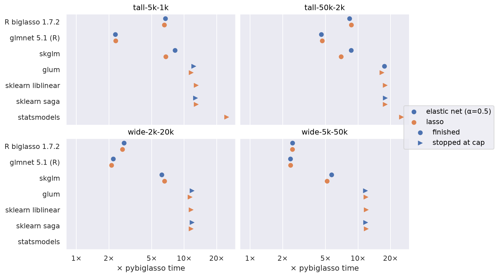
Which solvers. R biglasso, the original; R's glmnet, whose coordinate descent biglasso builds on; and every maintained Python package, installable with pip, that fits L1 or elastic-net logistic regression on a CPU: scikit-learn (its liblinear and saga solvers), glum, skglm, and statsmodels.
Other Python solvers. Each competitor was stopped once it took 10x as long as pybiglasso, which would otherwise have stretched the run to many hours. (The cap was set by an earlier, slower pybiglasso; measured against the one timed here, the caps fall at 11–25x, and glum's one finish, the 50,000 x 2,000 elastic net on 12 threads, is at 18x.) Only skglm finishes within that on every dataset, at 5–7x for the lasso and 6–9x for the elastic net. statsmodels (lasso only) ran only on the tall datasets: its L1 fit uses a general-purpose optimizer with dense matrices over twice the columns, which would need about 12 GB and 76 GB on the wide ones. To show how large the gaps get, the smallest problem (5,000 x 1,000) also ran with no cap:
| Solver | Lasso | Elastic net (α=0.5) | Worst relative suboptimality |
|---|---|---|---|
| pybiglasso | 0.60 s | 0.60 s | 1e-6 |
pybiglasso, eps=1e-10 |
1.37 s | 1.34 s | 3e-10 |
| glmnet 5.1 (R) | 1.4 s (2.3x) | 1.4 s (2.4x) | 2e-6 |
| skglm | 4.1 s (7x) | 4.4 s (7x) | 2e-4 |
| glum, 6 threads | 9.6 s (16x) | 10.9 s (18x) | 6e-9 |
| sklearn liblinear | 20.5 s (34x) | — | 5e-6 |
| sklearn saga | 90.7 s (151x) | 94.8 s (157x) | 1e-5 |
| statsmodels | over 900 s (over 1,000x) | — | — |
R biglasso 1.7.2. Times are in seconds; "best" is each package at its
fastest thread count. For the lasso, both packages fit identical paths. For the
elastic net, each ran its own update (see
Differences); pybiglasso with
r_compatible=True, which matches R, takes about as long as its default.
| Dataset | Penalty | pybiglasso, 1 thread | R, 1 thread | pybiglasso, best | R, best | Speedup (best) |
|---|---|---|---|---|---|---|
| 5,000 x 1,000 | lasso | 0.62 | 4.06 | 0.60 | 3.92 | 6.5x |
| 5,000 x 1,000 | elastic net | 0.63 | 4.17 | 0.60 | 4.04 | 6.7x |
| 50,000 x 2,000 | lasso | 9.31 | 55.7 | 6.23 | 54.1 | 8.7x |
| 50,000 x 2,000 | elastic net | 9.35 | 56.1 | 6.32 | 52.9 | 8.4x |
| 2,000 x 20,000 | lasso | 1.23 | 4.71 | 1.08 | 2.90 | 2.7x |
| 2,000 x 20,000 | elastic net | 1.31 | 4.80 | 1.08 | 2.99 | 2.8x |
| 5,000 x 50,000 | lasso | 7.45 | 27.2 | 6.29 | 15.5 | 2.5x |
| 5,000 x 50,000 | elastic net | 7.43 | 27.5 | 6.42 | 15.9 | 2.5x |
R's adaptive screening rule is no faster than SSR on these problems.
glmnet 5.1. glmnet standardized X itself (standardize = TRUE, its
default), as pybiglasso does, so both times include standardizing; the Python
solvers, which don't standardize, were given X already standardized. glmnet fit
with an intercept, along the same lambda grid, at its default tolerance; it runs
on one thread. Its objective is the benchmark's. It fit every path in full, at
2.1–4.7x pybiglasso's best time (1.8–3.1x pybiglasso's on one thread), and about as accurately: a worst relative suboptimality of 2e-8
to 3e-6, against pybiglasso's 6e-8 to 3e-6.
Out of core
This test fits a 12 GB float64 matrix (20,000 x 75,000) with
memory capped at 3 GB. pybiglasso read a numpy memmap under a cgroup memory
limit; R read a file-backed big.matrix in a container with the same limit,
and both were measured from their cgroup's accounting. Before each run, the
matrix was evicted from the page cache. Both fit the same 20-lambda lasso path
and agree to 1e-9, with identical iteration counts. pybiglasso ran twice, and
both runs are shown; R ran once.
| Fit time | Peak memory | Re-read from disk during the fit | |
|---|---|---|---|
| pybiglasso, 1 thread | 111 s, 131 s | 3.2 GB (at the cap) | 7.9 GB, 10.9 GB |
| pybiglasso, 6 threads | 109 s, 151 s | 3.2 GB (at the cap) | 13.3 GB, 15.1 GB |
| R biglasso 1.7.2 | 148 s, plus 41 s to build the big.matrix |
3.2 GB (at the cap) | 10.6 GB |
Here the disk sets the pace, and times vary by a third from run to run. Extra threads don't reliably help: they evict pages each other still need.
Not compared
Some solvers fall outside the rule above:
- Other languages: Julia's GLMNet.jl, a wrapper of glmnet's earlier Fortran solver, and Lasso.jl, written in Julia.
- Other hardware: RAPIDS cuML fits on a GPU, and only data that fits in GPU memory.
- Unmaintained: python-glmnet, archived, with its last release in 2020.
- A different problem: celer's logistic regression fits the lasso only, and no intercept. skglm, from the same authors, fits an intercept and the elastic net, and is compared above.
- Not a solver: benchopt is a benchmarking framework; its logistic-regression benchmark fits without an intercept or standardization, which pybiglasso doesn't support yet.
Differences from R biglasso
pybiglasso follows R biglasso 1.7.2 closely, matching it coefficient for coefficient and down to its iteration and screening counts. It departs in a few places, mostly where we think R's behavior may not be what was intended; if we've erred we'd be glad to be corrected. Each departure is marked in the code with a comment beginning "Differs from R biglasso".
Both families.
- Zero penalty factors. With a
penalty.factorof 0 and the default lambda grid, R's grid comes out aslambda = 0at every step. pybiglasso instead fits the unpenalized columns first, and starts the path at the smallest lambda that keeps every penalized column at zero. - Default
lambda_min. R chooses 0.001 or 0.05 by comparingnrow(X)withncol(X); pybiglasso compares the number of rows actually fit, which differs whenrow_indicesis given. - Data far from zero. For columns whose mean is large next to their spread (say, values near 1e8 that vary by 1), standardizing from raw sums loses precision in floating point. R's scales, and so its fit, can be affected without a warning; in our tests some scales came out as NaN. pybiglasso computes these columns' moments from centered values, so a constant shift of X leaves the solution unchanged.
- Invalid input. NaN or infinite values in the rows being fit, and
non-finite penalty factors or lambdas, raise
ValueError; R instead drops the affected column or returns the null model. - Unrepresentable grids. If an automatic grid overflows (for example,
with extremely small positive
alpha), R returns non-finite penalties, and pybiglasso raisesValueError, for both families and in both modes. Finite supplied grids remain supported, including in compatibility mode.
Least squares.
- Constant responses. R's strict convergence comparison against
a zero null loss uses the full iteration budget for a constant response.
pybiglasso stops once the coefficients no longer change;
r_compatible=Trueretains R's comparison. - Zero maximum penalty. R's logarithmic grid calculation can produce non-finite values when the maximum penalty is zero. pybiglasso returns a finite all-zero grid, whose fits solve the unpenalized problem.
- Loss after an iteration limit. R can leave
lossat zero when the budget ends with outstanding KKT violations. pybiglasso reports the returned model's residual sum of squares;r_compatible=Trueretains R's bookkeeping.
Logistic regression.
- Elastic-net update. For
alpha < 1, R's logistic coordinate update divides byv * (1 + l2), where the elastic-net objective in its documentation calls forv + l2, so the two solve somewhat different problems. pybiglasso usesv + l2, as glmnet and scikit-learn do;r_compatible=Truereproduces R exactly for this update. - Probability clipping. R sets probabilities
to 0 or 1 beyond
|eta| > 10, with weights of1e-4. Default mode uses glmnet'spmin = 1e-9boundary,|eta| > log(1 / pmin - 1)(about 20.7). This reduces each clipped row's probability error from at most4.6e-5to1e-9. We retain a positive boundary weight ofpmin * (1 - pmin)so the working residual(y - p) / wremains defined; glmnet can use zero weights. Default-mode coefficients, iterations and screening counts can change, for both lasso and elastic net.r_compatible=Trueretains R's cutoff and weights. Independent KKT checks against pinned glmnet fits cover the change. - Deviance.
devianceis the deviance, -2 log-likelihood, of the returned model. R reportsloss, half the deviance, computed before the final coordinate sweep and with probabilities clipped at 0 and 1, so it can occasionally be infinite.r_compatible=Truekeeps R's version. - Saturation.
stop_on_saturation=False, an option R doesn't have, fits every lambda, even past R's saturation cutoff.
Threads, cross-validation, and storage
pybiglasso reads the matrix one column at a time, through the memmap, and never loads or copies it; strong-rule screening skips most columns at most steps. Cross-validation folds are row indices into the same matrix on disk.
- Threads help larger fits (
n_threads=). Coordinate descent updates one coefficient at a time, so the sweep itself is sequential; the screening and optimality scans run in parallel across columns, and on tall data the logistic fits' per-row IRLS step runs in parallel across rows. Small problems gain little, larger ones more: on the 50,000 x 2,000 logistic benchmark, the fastest thread count takes two-thirds the time of one (see Performance). Out of core, threads can help when memory to spare holds the page cache, by keeping more disk reads in flight; under a tight memory limit they hurt, so usen_threads=1there. Results are bit-identical at any thread count. - Cross-validation scales with cores.
BiglassoRegressorCV(n_jobs=...)andBiglassoClassifierCV(n_jobs=...)fit folds in parallel threads that share one X (and, for a memmap, one page cache); results don't depend onn_jobs. - Cross-validation can stop each fold early. With
BiglassoClassifierCV(early_stopping=10), a fold's path stops once its held-out score has gone 10 alphas without improving, as bigstatsr'sbig_spLogRegdoes, and the fit on all the rows stops at the chosen alpha. On wide data, where the end of the path costs most, this saves much of the work; the cost is that a better score past the stopping point goes unseen. It is off by default. - Store X compactly. Since the work is mostly moving bytes, a narrower
dtype is faster: small integers (counts, categories, 0/1 indicators) as
int8oruint8take 8x less memory and disk than float64, and fit 1.3–1.6x faster in memory;float32halves the memory and is about as fast. Each value is read as a float64, so values that a narrower dtype holds exactly give bit-identical results. - Bounds checking is on by default. Every index into an array is checked,
which guards against a bug in pybiglasso reading past the end of X (inputs,
row_indicesamong them, are validated before a fit either way). It costs little where X's rows are read in place: a whole Fortran-ordered X, or a subset of at least half its rows without repeats, as in cross-validation, which is read through a mask. Where every read goes through an index or a stride (C-ordered X, or a smaller or repeatingrow_indices), it costs up to about 15%.PYBIGLASSO_BOUNDSCHECK=0turns it off; the path is the same (lambdas, iterations, screening), with identical coefficients.
How the code is organized
R biglasso implements each family's solver in a few long C++ functions; for
logistic regression, two:
cdfit_binomial_ssr standardizes, sets up the lambda grid, and runs the lambda
loop with its strong rule and KKT checks, and cdfit_binomial_lambda_core runs
the coordinate descent at each lambda. That keeps the algorithm in a few places,
close to how it's written in the papers.
pybiglasso splits the same algorithm into one small function per step, each
documenting the state it changes, plus a short driver, fit_lambda, that reads
like the algorithm's outline. To my eye that's easier to read, test, and modify.
It's a matter of taste, though; some excellent programmers prefer the long
inlined function you can read straight through (John Carmack has
a good essay on
why). The solver takes the same number of iterations as R's at every lambda; the
R comparison checks this in every case.
The solver is written twice, in the same steps. The one that runs is Rust
(rust/src/solver.rs): one call from Python fits the whole path. The readable one,
tests/support/reference.py, is plain numpy,
step by step, and imports nothing from pybiglasso; the tests hold the Rust
solver to it, and both to R.
pybiglasso (rust/src/solver.rs) |
R biglasso (src/) |
|---|---|
center_scale, compute_z |
standardize_and_get_residual (utilities.cpp) |
update_irls |
probability and weight update in cdfit_binomial_lambda_core (binomial.cpp) |
update_intercept |
intercept update in cdfit_binomial_lambda_core |
coordinate_sweep (Pass) |
coordinate loop in cdfit_binomial_lambda_core; wcrossprod_resid, wsqsum_bm, lasso (utilities.cpp) |
check |
check_strong_set, check_rest_set (utilities.cpp) |
fit_lambda |
cdfit_binomial_lambda_core |
run |
cdfit_binomial_ssr |
The least-squares driver and coordinate sweeps, in rust/src/gaussian.rs, port
R's Gaussian SSR solver the same way. They share column access,
standardization, and the fixed-order sums with the logistic solver, and since
the curvature is constant they update residuals directly, without the IRLS
step. The numpy reference covers both families.
Every sum over rows runs in an order fixed by the data's shape alone. Threads split the work by column, and a tall column's rows into 2,048-row chunks whose sums are added in order. Within a chunk, eight running sums are combined in a fixed order, so vector instructions of any width (AVX2, AVX-512, ARM's NEON) give the same result, and no multiply and add are fused into one instruction, which would round differently. Exponentials and logarithms come from a portable implementation rather than the operating system's math library, whose last bits differ between Linux, macOS, and Windows. So results are bit-identical at any thread count, on any CPU, and on every operating system with a wheel.
Scope
- Gaussian (least-squares) and binomial (logistic) families; Cox is not ported.
- SSR (sequential strong rule) screening only. R uses its newer Hybrid and Adaptive rules only for the plain lasso without penalty factors, and they were no faster than SSR on our benchmarks.
Citation
Zeng Y, Breheny P (2021). The biglasso Package: A Memory- and Computation-Efficient Solver for Lasso Model Fitting with Big Data in R. The R Journal, 12(2), 6–19. doi:10.32614/RJ-2021-001
License
GPL-3.0-or-later, as R biglasso is GPL-3.
1 maintainer

Metadata
1 maintainer
Release files for pybiglasso 0.4.0
For a detailed explanation of source distributions (sdists) and built distributions (wheels), please see the package formats documentation.
Source distribution (sdist)
| File | Size | Uploaded | Provenance | Actions |
|---|---|---|---|---|
| pybiglasso-0.4.0.tar.gz | 1.1 MB | With provenance | Details for pybiglasso-0.4.0.tar.gz |
Built distributions (wheels)
| File | Actions Reset | |||
|---|---|---|---|---|
| pybiglasso-0.4.0-cp311-abi3-win_amd64.whl | CPython 3.11 | abi3 | Windows x86-64 | Details for pybiglasso-0.4.0-cp311-abi3-win_amd64.whl |
| pybiglasso-0.4.0-cp311-abi3-manylinux_2_17_x86_64.manylinux2014_x86_64.whl | CPython 3.11 | abi3 | Linux glibc 2.17+ x86-64 | Details for pybiglasso-0.4.0-cp311-abi3-manylinux_2_17_x86_64.manylinux2014_x86_64.whl |
| pybiglasso-0.4.0-cp311-abi3-manylinux_2_17_aarch64.manylinux2014_aarch64.whl | CPython 3.11 | abi3 | Linux glibc 2.17+ ARM64 | Details for pybiglasso-0.4.0-cp311-abi3-manylinux_2_17_aarch64.manylinux2014_aarch64.whl |
| pybiglasso-0.4.0-cp311-abi3-macosx_11_0_arm64.whl | CPython 3.11 | abi3 | macOS 11.0+ ARM64 | Details for pybiglasso-0.4.0-cp311-abi3-macosx_11_0_arm64.whl |
| pybiglasso-0.4.0-cp311-abi3-macosx_10_12_x86_64.whl | CPython 3.11 | abi3 | macOS 10.12+ x86-64 | Details for pybiglasso-0.4.0-cp311-abi3-macosx_10_12_x86_64.whl |
Total release size: 17.8 MB
Release files / pybiglasso-0.4.0.tar.gz
| Download URL | pybiglasso-0.4.0.tar.gz |
|---|---|
| Size | 1.1 MB |
| Tags | Source |
|
SHA-256 checksum How to use checksums |
bd76a1ca3a79cd9fcb5dc156a2f5f1e11f39b01071dc38579f2bd737511c7803
|
|
BLAKE2b-256 checksum How to use checksums |
02ee4bee1c9be936f9e9bc60a3adfeeac2945591765f085e031f39ffee6b4b14
|
| Upload date | |
|
Uploaded using Trusted Publishing? What is trusted publishing? |
Yes |
| Uploaded via |
twine/7.0.0 CPython/3.13.16
|
Provenance
Provenance describes where a file came from. On PyPI, provenance is shared via attestations, which provide a verifiable record of the build or publishing details. View details, limitations and caveats.


PyPI Publish Attestation
PyPI verified that this artifact, at this checksum, originated from the publisher listed below.
Signed by GitHub Actions, verified by PyPI on Oct 28, 2026.
Transparency logRelease files / pybiglasso-0.4.0-cp311-abi3-win_amd64.whl
| Download URL | pybiglasso-0.4.0-cp311-abi3-win_amd64.whl |
|---|---|
| Size | 4.2 MB |
| Tags | CPython 3.11 Windows x86-64 abi3 |
|
SHA-256 checksum How to use checksums |
d418d595440409a818339605b534e9fd32142af467fd94e7661d58cf32931e38
|
|
BLAKE2b-256 checksum How to use checksums |
3434be5594b7bbb5e3fbf5a86666c430b3dc801a35b0c49688cebee6cd262738
|
| Upload date | |
|
Uploaded using Trusted Publishing? What is trusted publishing? |
Yes |
| Uploaded via |
twine/7.0.0 CPython/3.13.16
|
Provenance
Provenance describes where a file came from. On PyPI, provenance is shared via attestations, which provide a verifiable record of the build or publishing details. View details, limitations and caveats.
PyPI Publish Attestation
PyPI verified that this artifact, at this checksum, originated from the publisher listed below.
Signed by GitHub Actions, verified by PyPI on Oct 28, 2026.
Transparency logRelease files / pybiglasso-0.4.0-cp311-abi3-manylinux_2_17_x86_64.manylinux2014_x86_64.whl
| Download URL | pybiglasso-0.4.0-cp311-abi3-manylinux_2_17_x86_64.manylinux2014_x86_64.whl |
|---|---|
| Size | 4.0 MB |
| Tags | CPython 3.11 Linux glibc 2.17+ x86-64 abi3 |
|
SHA-256 checksum How to use checksums |
ed9a7ef254211160b7a647cdcb8ee5f3fe3408d7401d4ea78e0f83d0b8c22f95
|
|
BLAKE2b-256 checksum How to use checksums |
f67c0b17f747b73e96d2762e961a4b94d7dbd32f028c2e88b36eb62beb671bc0
|
| Upload date | |
|
Uploaded using Trusted Publishing? What is trusted publishing? |
Yes |
| Uploaded via |
twine/7.0.0 CPython/3.13.16
|
Provenance
Provenance describes where a file came from. On PyPI, provenance is shared via attestations, which provide a verifiable record of the build or publishing details. View details, limitations and caveats.
PyPI Publish Attestation
PyPI verified that this artifact, at this checksum, originated from the publisher listed below.
Signed by GitHub Actions, verified by PyPI on Oct 28, 2026.
Transparency logRelease files / pybiglasso-0.4.0-cp311-abi3-manylinux_2_17_aarch64.manylinux2014_aarch64.whl
| Download URL | pybiglasso-0.4.0-cp311-abi3-manylinux_2_17_aarch64.manylinux2014_aarch64.whl |
|---|---|
| Size | 2.4 MB |
| Tags | CPython 3.11 Linux glibc 2.17+ ARM64 abi3 |
|
SHA-256 checksum How to use checksums |
0f4a6b3ff48891e1766123e05473993b4f220cc7de1cbe1f078191799c4aef13
|
|
BLAKE2b-256 checksum How to use checksums |
055c3bdc2957e68f757d3969220fe7c56f3534ba584ae81a6908c299d0c0cea0
|
| Upload date | |
|
Uploaded using Trusted Publishing? What is trusted publishing? |
Yes |
| Uploaded via |
twine/7.0.0 CPython/3.13.16
|
Provenance
Provenance describes where a file came from. On PyPI, provenance is shared via attestations, which provide a verifiable record of the build or publishing details. View details, limitations and caveats.
PyPI Publish Attestation
PyPI verified that this artifact, at this checksum, originated from the publisher listed below.
Signed by GitHub Actions, verified by PyPI on Oct 28, 2026.
Transparency logRelease files / pybiglasso-0.4.0-cp311-abi3-macosx_11_0_arm64.whl
| Download URL | pybiglasso-0.4.0-cp311-abi3-macosx_11_0_arm64.whl |
|---|---|
| Size | 2.4 MB |
| Tags | CPython 3.11 abi3 macOS 11.0+ ARM64 |
|
SHA-256 checksum How to use checksums |
aea8cffd6568de7574392f009e1edd64f7fe9d1df9658931c586258b328b2ee1
|
|
BLAKE2b-256 checksum How to use checksums |
303043b03914ec28d3df90d5f31fb695a98e0571fdf430989d8a870ae8112162
|
| Upload date | |
|
Uploaded using Trusted Publishing? What is trusted publishing? |
Yes |
| Uploaded via |
twine/7.0.0 CPython/3.13.16
|
Provenance
Provenance describes where a file came from. On PyPI, provenance is shared via attestations, which provide a verifiable record of the build or publishing details. View details, limitations and caveats.
PyPI Publish Attestation
PyPI verified that this artifact, at this checksum, originated from the publisher listed below.
Signed by GitHub Actions, verified by PyPI on Oct 28, 2026.
Transparency logRelease files / pybiglasso-0.4.0-cp311-abi3-macosx_10_12_x86_64.whl
| Download URL | pybiglasso-0.4.0-cp311-abi3-macosx_10_12_x86_64.whl |
|---|---|
| Size | 3.8 MB |
| Tags | CPython 3.11 abi3 macOS 10.12+ x86-64 |
|
SHA-256 checksum How to use checksums |
32d5cfd07d2aee380eee4e356f51ffcb239f99497ce79a19651c58ad80ed2072
|
|
BLAKE2b-256 checksum How to use checksums |
f8067428ccc2d13d3506e0e3153f049d02b3ee4db17a4a1b81e17d4e7475042f
|
| Upload date | |
|
Uploaded using Trusted Publishing? What is trusted publishing? |
Yes |
| Uploaded via |
twine/7.0.0 CPython/3.13.16
|
Provenance
Provenance describes where a file came from. On PyPI, provenance is shared via attestations, which provide a verifiable record of the build or publishing details. View details, limitations and caveats.
PyPI Publish Attestation
PyPI verified that this artifact, at this checksum, originated from the publisher listed below.
Signed by GitHub Actions, verified by PyPI on Oct 28, 2026.
Transparency logSecurity for pybiglasso 0.4.0
Provenance
Provenance describes where a file came from. On PyPI, provenance is shared via attestations, which provide a verifiable record of the build or publishing details. View details, limitations and caveats.
Full provenance
All 6 files in this release have been uploaded with provenance metadata.
Attestation for pybiglasso-0.4.0.tar.gz
PyPI Publish Attestation
PyPI verified that this artifact, at this checksum, originated from the publisher listed below.
Signed by GitHub Actions, verified by PyPI on Oct 28, 2026.
Transparency logA note on package security
PyPI is a repository for distributing packages, not a service for auditing them. While third-party security researchers and our staff do their best to detect and remove malicious packages, PyPI cannot guarantee the quality, security or suitability of any given package.
To learn more about protecting yourself from malicious actors, visit our package security documentation.














