Boundary fits using polynomials or splines

Project description
pyboundfit
Boundary fits using polynomials or splines, based on the method described in Cardiel 2009. This code is a Python implementation of part of the functionality implemented in the original Fortran 77 code boundfit.
The numerical minimization of the fit to splines is performed with the help of the package lmfit.
Warning: this code is under development. Major changes are still being introduced.
Instaling the code
In order to keep your Python installation clean, it is highly recommended to first build a specific Python 3 virtual enviroment
Creating and activating the Python virtual environment
$ python3 -m venv venv_pyboundfit
$ . venv_pyboundfit/bin/activate
(venv_pyboundfit) $
Installing the package
The latest stable version is available via de PyPI repository:
(venv_pyboundfit) $ pip install pyboundfit
Note: This command can also be employed in a Windows terminal opened through the
CMD.exe prompt icon available in Anaconda Navigator.
The latest development version is available through GitHub:
(venv_pyboundfit) $ pip install git+https://github.com/nicocardiel/pyboundfit.git@main#egg=pyboundfit
Testing the installation
(venv_pyboundfit) $ pip show pyboundfit
(venv_pyboundfit) $ ipython
In [1]: import pyboundfit
In [2]: print(pyboundfit.__version__)
0.3.0
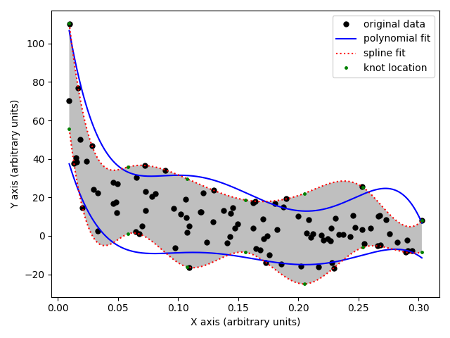
In [3]: pol1, pol2, spl1, spl2 = pyboundfit.demo()
Computing upper boundary (polynomial fit)... OK!
Computing lower boundary (polynomial fit)... OK!
Computing upper boundary (splines fit)... OK!
Computing lower boundary (splines fit)... OK!
In [4]: pol1.coef
Out[4]:
array([ 22.43919975, -41.5216713 , -7.32451917, 140.23297889,
41.59855497, -148.66578342])
...
The demo function computes the boundary fits to some example data and
generates the following plot:
Usage
Import the required packages
import matplotlib.pyplot as plt
import numpy as np
import pyboundfit as bf
Generate some random data to be fitted
npoints = 300
rng = np.random.default_rng(seed=1234)
xfit = np.linspace(1.0, 3.5, npoints)
yfit = np.sin(xfit) + rng.normal(loc=0, scale=0.1, size=npoints)
Fit upper and lower boundaries using polynomials
pol_upper = bf.boundfit_poly(
    x=xfit, y=yfit, deg=5,
    xi=10, niter=100, expweight=True,
    boundary='upper'
)
pol_lower = bf.boundfit_poly(
    x=xfit, y=yfit, deg=5,
    xi=10, niter=100, expweight=True,
    boundary='lower'
)
Fit upper and lower boundaries using splines (the numerical minimization takes some time).
spl_upper = bf.boundfit_adaptive_splines(
    x=xfit, y=yfit, t=5,
    xi=100, niter=100, boundary='upper',
    adaptive=False,
    expweight=True
)
spl_lower = bf.boundfit_adaptive_splines(
    x=xfit, y=yfit, t=5,
    xi=100, niter=100, boundary='lower',
    adaptive=False,
    expweight=True
)
Display the result
import matplotlib.pyplot as plt
fig, ax = plt.subplots()
ax.plot(xfit, yfit, 'ko')
ax.plot(xfit, pol_upper(xfit), '-', label='upper boundary (polynomial)')
ax.plot(xfit, pol_lower(xfit), '-', label='lower boundary (polynomial)')
ax.plot(xfit, spl_upper(xfit), ':', label='upper boundary (splines)')
ax.plot(xfit, spl_lower(xfit), ':', label='lower boundary (splines)')
ax.set_xlabel('X axis')
ax.set_ylabel('Y axis')
ax.legend()
plt.tight_layout()
plt.show()
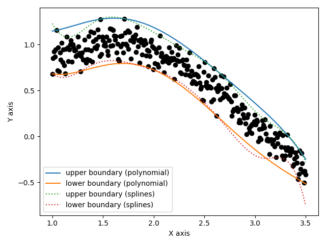
Please, note that the results are quite sensitive to the fitting parameters.
Citation
If you find this package useful, please cite Cardiel 2009.
@ARTICLE{2009MNRAS.396..680C,
       author = {{Cardiel}, N.},
        title = "{Data boundary fitting using a generalized least-squares method}",
      journal = {\mnras},
     keywords = {methods: data analysis, methods: numerical, Astrophysics - Instrumentation and Methods for Astrophysics},
         year = 2009,
        month = jun,
       volume = {396},
       number = {2},
        pages = {680-695},
          doi = {10.1111/j.1365-2966.2009.14749.x},
archivePrefix = {arXiv},
       eprint = {0903.2068},
 primaryClass = {astro-ph.IM},
       adsurl = {https://ui.adsabs.harvard.edu/abs/2009MNRAS.396..680C},
      adsnote = {Provided by the SAO/NASA Astrophysics Data Syste
Release history Release notifications | RSS feed


Download files
Download the file for your platform. If you're not sure which to choose, learn more about installing packages.
Source Distribution
Built Distribution
Filter files by name, interpreter, ABI, and platform.
If you're not sure about the file name format, learn more about wheel file names.
Copy a direct link to the current filters
File details
Details for the file pyboundfit-0.3.0.tar.gz.
File metadata
- Download URL: pyboundfit-0.3.0.tar.gz
- Upload date:
- Size: 24.8 kB
- Tags: Source
- Uploaded using Trusted Publishing? No
- Uploaded via: twine/6.1.0 CPython/3.12.7
File hashes
| Algorithm | Hash digest | |
|---|---|---|
| SHA256 |
7cae7f5f99067809ab9e9523c110c4c47be74be7d1c4d3fa33629aa1ffa005db
|
|
| MD5 |
568778bc329bf51b31d4d4e756743e03
|
|
| BLAKE2b-256 |
790abef96ff431190e00027d7cf7ad7b96802c58c0070a656cec0308798ccc22
|
File details
Details for the file pyboundfit-0.3.0-py3-none-any.whl.
File metadata
- Download URL: pyboundfit-0.3.0-py3-none-any.whl
- Upload date:
- Size: 25.8 kB
- Tags: Python 3
- Uploaded using Trusted Publishing? No
- Uploaded via: twine/6.1.0 CPython/3.12.7
File hashes
| Algorithm | Hash digest | |
|---|---|---|
| SHA256 |
7f1be5fdf6f372aa3dc600ea6cf8dbf273f180ed412e7cab2a989e8d40148472
|
|
| MD5 |
e605cb5012499a6d35b3f3c47ba51c3b
|
|
| BLAKE2b-256 |
1bc60269b4207c81a3b97eeb51c110ea65d75b9b561dfd037ee700ce76d37dc8
|


