Complexity Measures and Visualization for Image datasets

Project description

pycol-vis: Python Image Complexity Library
The Python Image Complexity Library (pycol-vis) assembles a set of data complexity measures associated with image data.
Dataset complexity poses a significant challenge in classification tasks, especially in real-world applications where a combination of factors such as class overlap, data imbalance, noise, and dimensionality can jeopardize a machine learning algorithm's performance.
The seminal work of [1] has leveraged a set of measures devoted to estimating the difficulty level of a tabular classification problem. However, since these complexity measures were designed for tabular datasets, they cannot be directly applied to images. Furthermore, while comprehensive software packages for complexity analysis exist for tabular data such as pycol , dcol , ECoL, ImbCoL, SCoL, and mfe no equivalent, standardized toolkit exists for image datasets.
The lack of dedicated image measures and the absence of supporting software, have created a significant gap in our understanding of image complexity, despite the importance of image data in areas such as healthcare, security, remote sensing, and autonomous systems. Our work aims to address this gap directly by introducing a comprehensive package for this purpose. In particular, the pycol-vis package distinguishes itself by categorizing image metrics into two distinct complexity families:
- Intrinsic: comprised of metrics to quantify the difficulty of individual images, based image properties such as color, entropy and edge density.
- Overlap: focusing on class separability and complexity between classes, of a binary or multiclass image dataset.
Implemented Measures
The following Table shows the measures implemented in our package divided by family:
| Category | Name | Acronym | Range | Reference |
|---|---|---|---|---|
| Overlap | Cumulative Spectral Gradient | CSG | 0–∞ | [2] |
| Overlap | Area Under Laplacian Spectrum | AULS | 0–∞ | [3] |
| Overlap | Cumulative Maximum Scaled Area Under Laplacian Spectrum | cmsAULS | 0–∞ | [3] |
| Overlap | Class Separability | m-sep | 0–∞ | [4] |
| Overlap | In-Class Variability | m-var | 0–∞ | [4] |
| Intrinsic | JPEG Compression Ratio | JPEG | 0–1 | [5] |
| Intrinsic | Fractal Compression | Fractal | 0–1 | [5] |
| Intrinsic | Entropy | H | 0–1 | [6] |
| Intrinsic | Canny Edge Density | CED | 0–1 | [7] |
| Intrinsic | Sobel Edge Density | SED | 0–1 | [7] |
| Intrinsic | Color Average/STD | Color Avg. | [0–1, 0–1, 0–1] | [6] |
| Intrinsic | Unique Colors | #Colors | 1–∞ | [7] |
| Intrinsic | Zipf Rank/Difference | Zipf | 0–1 | [5] |
| Intrinsic | Haralick Features | haralick | 0-1 | [7] |
| Intrinsic | FFT Features | fft | 0-1 | — |
Overlap Measures
- Cumulative Spectral Gradient (CSG): Graph-based measure derived from spectral clustering, representing the minimum cutting cost of the similarity matrix.
- Area Under Laplacian Spectrum (AULS): Measures the area under the Laplacian spectrum of the similarity graph.
- Cumulative Maximum Scaled AULS (cmAULS): Combines the CSG and AULS measures to capture different aspects of graph-based overlap.
- Class Separability (m-sep): Inter-class separability measure based on Linear Discriminant Analysis (LDA).
- In-Class Variability (m-var): Intra-class variability measure based on Linear Discriminant Analysis (LDA).
Intrinsic Measures
- JPEG Compression Ratio: Compression ratio obtained by compressing the image in JPEG format (compression quality is configurable).
- Fractal Compression: Compression ratio obtained using fractal image compression.
- Entropy: Shannon entropy of the image, measuring the amount of information or randomness.
- Edge Density (Canny/Sobel): Density of edges detected using either Canny or Sobel filters; higher density indicates higher visual complexity.
- Color Statistics (Mean / Std): Mean and standard deviation of pixel values for each color channel; images may be converted to different color spaces.
- Unique Colors: Number of unique colors after color quantization, capturing color diversity within the image.
- Zipf Rank / Difference: Complexity measure based on Zipf-like statistics, where the frequency of elements is inversely proportional to their rank.
- Haralick Features: Texture-based complexity measures derived from the Gray-Level Co-occurrence Matrix (GLCM).
- FFT Features: Frequency-based measures obtained by transforming the image into the frequency domain and computing the energy in low, mid, and high frequency bands.
Installation Instructions
All packages required to run pycol-vis are listed in the requirements.txt file found in this github repository. To install all needed packages run:
# Clone the repository
git clone https://github.com/DiogoApostolo/pycol-vis.git
cd pycol-vis

# Install dependencies
pip install -r requirements.txt

# Install the package in editable mode
pip install -e .
Alternatively, the package is also available for installation through pypi in pycol-vis:
pip install pycol-vis
⚠️ Note: pycol-vis requires Python 3.10, 3.11, or 3.12. Python 3.13 and newer are not currently supported due to TensorFlow compatibility.
Datasets
Below is a list of some of the datasets used to test our package which are also necessary to run the use case files:
- Shapes dataset: Dataset is composed of 2D 9 geometric shapes, each shape is drawn randomly on a 200x200 RGB image. (also available in shapes_dataset.zip)
- COVID Dataset: Covid Dataset with 3 classes COVID19, PNEUMONIA and NORMAL
- Fruits Dataset: A dataset contains 100 classes of fruit images. (also available in Fruit_dataset.zip)
- MNIST: A dataset of handwritten digits
- Fashion MNIST: A dataset of 28x28 pixel images of 10 fashion categories (e.g., shirts, shoes, bags)
This package expects the datasets to be stored in the following structure:
- Folder
- Class_1
- img1.png
- img2.png
- Class_2
- img1.png
- img2.png
- Class_1
Basic Usage
This section shows how to correctly import the package, load a dataset, parameterize the setup and extract dataset complexity.
from pycol_vis.image_metrics import ImageComplexity

# Load the Dataset Stored in the Fruits folder, keeping only the apple and banana class and 100 samples (selected randomly) from each class.
comp = ImageComplexity('Fruits',
           keep_classes=['apple',
           'banana'],
           number_per_class=100)

#Calculate the CSG overlap Measure and the JPEG Compression measure and print them to the user
print(comp.csg_measure())
print(comp.jpeg_compression_ratio())


#Example of the CSG parameters, specifying a specific embedding and how many samples to use to estimate probability.
comp.csg_measure(
    emb_type="mobile_net",
    n_samples=50
)
Visualization Example
Our package offers the user diverse methods to visualize dataset complexity.
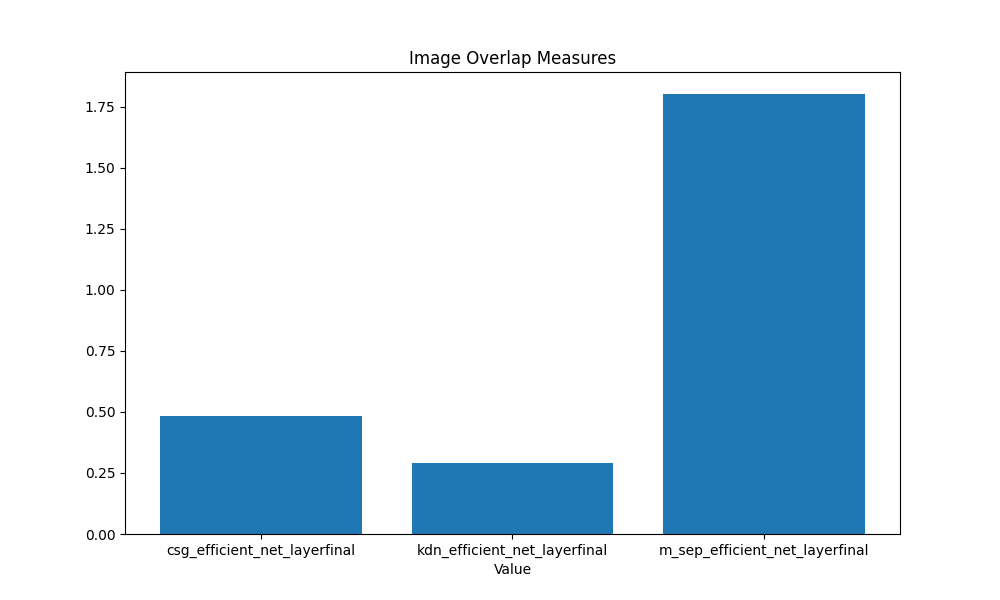
This example shows how the measured overlap complexity can be show in a bar plot. The plot_overlap_measures function automatically grabs all overlap measures calculated until that point and displays them to the user.
#Load Dataset

dataset = "shapes_dataset"
folder = "./" + dataset +  "/train/"
classes = ["Circle","Square","Triangle"]


complexity = ImageComplexity(folder,keep_classes=classes,number_per_class=200)

# Measure Complexity
complexity.csg_measure(emb_type="efficient_net",n_samples=50, reduction_type='pca')
complexity.tabular_measure(emb_type='efficient_net',measure='kdn',reduction_type='pca')
complexity.m_sep_measure(emb_type='efficient_net', reduction_type='pca')

#Plot Bar plot with measured complexity
complexity.plot_overlap_measures()
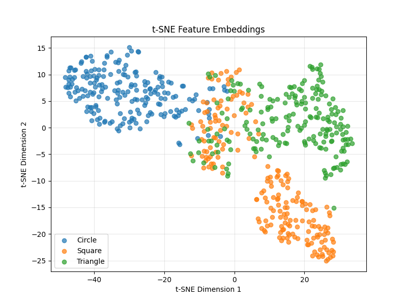
Continuing from the previous example, a user might also want to visualize how the dataset was embedded. Using the plot_tsne method our package uses t-SNE to show the user a 2D projection of the embedded dataset.
complexity_train.plot_tsne(embs=complexity_train.feature_embeddings)
Use Cases
A collection of Use Cases are provided in the use_cases folder. These examples display how our package can be used in practice to extract valuable insights from image datasets.
In particular de use case folder includes the following files:
- model_selection.py: A Use Case showing how the overlap measures in our package can be used to inform model selection
- sample_selection.py: A Use Case showing how the intrinsic measures can be used to reduce the dataset size, selecting only the most relevant samples
- dim_reduction.py: A Use Case showing how the overlap measures can be used to reduce the embedding feature space, without losing classification performance.
- viz_example.py: A Use Case displaying the different visualization options present in our package
- layers.py A Use Case of how to train a Custom NN and extract complexity at each layer.
More information is provided in each individual file.
References
[1] Ho, T. K., & Basu, M. (2002).
Complexity Measures of Supervised Classification Problems.
IEEE Transactions on Pattern Analysis and Machine Intelligence, 24(3), 289–300.
https://doi.org/10.1109/34.990132
[2] Branchaud-Charron, F., Achkar, A., & Jodoin, P.-M. (2019).
Spectral Metric for Dataset Complexity Assessment.
arXiv:1905.07299. https://arxiv.org/abs/1905.07299
[3] Li, G., Togo, R., Ogawa, T., & Haseyama, M. (2022).
Dataset complexity assessment based on cumulative maximum scaled area under Laplacian spectrum.
Multimedia Tools and Applications, 81(22), 32287–32303.
https://doi.org/10.1007/s11042-022-13027-3
[4] Cho, H., & Lee, S. (2021).
Data Quality Measures and Efficient Evaluation Algorithms for Large-Scale High-Dimensional Data.
Applied Sciences, 11(2), 472.
https://doi.org/10.3390/app11020472
[5] Machado, P., Romero, J., Nadal, M., Santos, A., Correia, J., & Carballal, A. (2015).
Computerized measures of visual complexity.
Acta Psychologica, 160, 43–57.
https://doi.org/10.1016/j.actpsy.2015.06.005
[6] Rahane, A. A., & Subramanian, A. (2020).
Measures of Complexity for Large Scale Image Datasets.
arXiv:2008.04431. https://arxiv.org/abs/2008.04431
[7] Corchs, S. E., Ciocca, G., Bricolo, E., & Gasparini, F. (2016).
Predicting Complexity Perception of Real World Images.
PLOS ONE, 11(6).
https://doi.org/10.1371/journal.pone.0157986
Release history Release notifications | RSS feed


Download files
Download the file for your platform. If you're not sure which to choose, learn more about installing packages.
Source Distribution
Built Distribution
Filter files by name, interpreter, ABI, and platform.
If you're not sure about the file name format, learn more about wheel file names.
Copy a direct link to the current filters
File details
Details for the file pycol_vis-0.2.7.tar.gz.
File metadata
- Download URL: pycol_vis-0.2.7.tar.gz
- Upload date:
- Size: 46.7 kB
- Tags: Source
- Uploaded using Trusted Publishing? No
- Uploaded via: twine/6.2.0 CPython/3.10.11
File hashes
| Algorithm | Hash digest | |
|---|---|---|
| SHA256 |
285bf0e10320541bebdce7ba72baf185b19efa251f8bceb5553e735fd29be6c5
|
|
| MD5 |
eecfe4e7f900940c538b6801ce3d5752
|
|
| BLAKE2b-256 |
0994d9ab470dae2c7a578c6ad0b0ece218331241226167d98bd3f85b9adb2fd6
|
File details
Details for the file pycol_vis-0.2.7-py3-none-any.whl.
File metadata
- Download URL: pycol_vis-0.2.7-py3-none-any.whl
- Upload date:
- Size: 49.9 kB
- Tags: Python 3
- Uploaded using Trusted Publishing? No
- Uploaded via: twine/6.2.0 CPython/3.10.11
File hashes
| Algorithm | Hash digest | |
|---|---|---|
| SHA256 |
540e19210fc8f6a190f5e053363c5aa0eb86dffe9df7a8fe94a1a6206fc48ba4
|
|
| MD5 |
2964309abd4ba676ed29f25c8edfc122
|
|
| BLAKE2b-256 |
b2b5131e7ae25a8c784b72531a2cabc527cea7901b70c1e9459f6857eaeb723f
|


