
🔭 pycream2
pycream2 is an AGN light curve fitting code that uses MCMC (via
JAX + NumPyro) to
model multi-band light curves as a lagged echo of a lamppost-driven
accretion disk1, inferring the posterior probability distributions of a
physically motivated disk model's parameters: accretion rate (mdot),
inclination, and temperature profile. Read on for install instructions,
tests on synthetic data, and example usage.
CREAM stands for Continuum Reprocessing AGN MCMC.
pycream2 is the successor to the original CREAM Fortran code and its
Python wrapper, pycecream:
a rewrite in pure JAX/NumPyro, with no Fortran compiler needed, gradient-based
(NUTS) sampling and a fast direct-solve mode.
pip install pycream2
If you use pycream2 in published work, please cite Starkey, Horne &
Villforth (2016): see 📝 Citing pycream2.
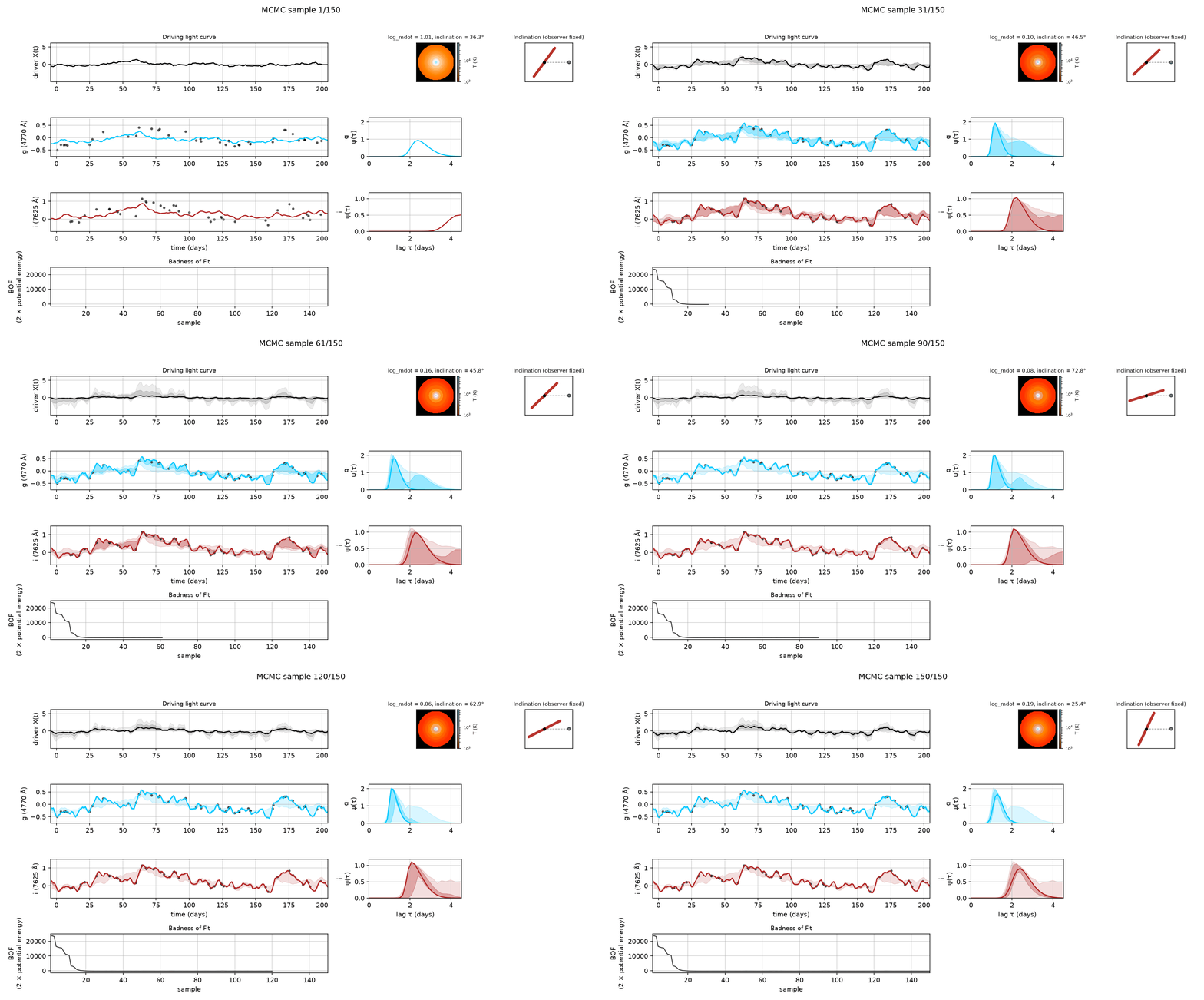
The driver, per-band echo/response-function fits (each with its own
68%/95% credible envelope, expanding cumulatively as more samples
accumulate -- wide early, narrowing as the chain converges), each band
coloured by its real-world wavelength (X-ray black, UV violet, visible its
actual spectral colour, IR+ reddish), a face-on disk-temperature view
with each ring drawn in the true blackbody colour of its temperature
(blue-white at the hot centre, orange-red in the cool outer disk, on a
fixed Kelvin colour bar; titled with the frame's current
log_mdot/inclination), and a side-on
schematic where the disk line tilts with inclination while the eye-on-a-
sphere observer and its line of sight stay fixed, and a Badness-of-Fit
trace growing one point per sample -- all early in a NUTS chain (short
warmup on purpose, so everything is still visibly finding its way).
Regenerate with python scripts/make_fit_animation.py.
🗂️ Contents
- 🔭 Background
- 🌀 Model
- 🧭 Choosing settings: the fitting guide
- 📦 Package layout
- ⚙️ Install
- 🚀 Quickstart
- 📈 Fitting your own light curves, with saved/resumable runs
- 🧪 Visual smoke test
- 📡 Real-data worked example: NGC 5548 (AGN STORM)
- ✅ Tests and coverage
- ⏱️ Performance profiling
- 🔄 Swapping the response function
- 🌈 Emission-line / free-lag mode and driver light curves
- ⚠️ Status / caveats
- 📝 Citing pycream2
🔭 Background
Active galactic nuclei (AGN) are powered by gas accreting onto a supermassive black hole through a hot, luminous disk. That disk doesn't shine steadily: its continuum flux flickers stochastically on timescales of days to months, and the flickering isn't synchronized across colour: shorter (bluer) wavelengths vary first, and longer (redder) wavelengths echo them with a delay of hours to days. The standard picture is a lamppost geometry: a compact, hard X-ray/UV-emitting corona above the disk irradiates it, each annulus reprocesses that irradiation and re-emits thermally at a wavelength set by its temperature (hotter, so bluer, closer in), and a cooler ring further out reprocesses more slowly, so its light reaches the observer later. The lag between bands is therefore a direct, geometry-independent probe of the disk's temperature profile and physical size.
Measuring those lags precisely (continuum reverberation mapping) is one of the few ways to measure an accretion disk's size directly, rather than inferring it from a spectral model, and it's turned out to be a genuinely useful stress test for disk theory: continuum RM campaigns (e.g. AGN STORM2, the SDSS Reverberation Mapping project3) have repeatedly found disks several times larger than standard thin-disk theory predicts for the same black hole mass and accretion rate: a persistent "disk size problem" that better lag measurements, not just better spectra, can help resolve.
It's a genuinely hard fitting problem, though: real light curves are noisy and irregularly sampled with observing gaps, and each band's flux is correlated red noise rather than independent points, so pairwise cross-correlation of light curves can be misleading, and what you really want is one joint statistical model of all bands at once that propagates uncertainty properly through to the physical parameters (black hole mass, accretion rate, inclination), not just to a best-fit lag per band pair.
pycream2 is a specific, opinionated take on that joint fit:
- Fully Bayesian, one model, every band at once. A single NumPyro model jointly infers the shared driving light curve, the disk response per band, and the physical parameters behind it, rather than fitting each band's lag independently and combining the results afterwards.
- Closed-form and differentiable. The driving light curve is represented as a finite Fourier series rather than a literal Gaussian process, which makes the disk-reprocessing convolution analytically closed-form (see "Model" below) instead of a numerical double integral; and because everything is written in JAX, gradients come for free, so fitting uses gradient-guided Hamiltonian Monte Carlo (NUTS) rather than a gradient-free sampler.
- Built for running a campaign, not just a demo script. Managed,
resumable fit runs (
EchoFit(title=...), checkpointing,EchoFit.resume()) and a one-command visual sanity-check report (scripts/smoke_test.py), because real fitting campaigns get interrupted midway and real results need to be eyeballed before they're trusted, not just produced.
This continues a line of continuum- and line-reverberation-mapping software (JAVELIN, PyROA, CREAM/MICA among others) rather than starting from nothing: see "Status / caveats" below for what hasn't been validated against real campaigns yet.
🌀 Model
Each band's observed light curve is modelled as
y_band(t) = S_band * ∫ X(t - τ) ψ(τ, λ_band, θ) dτ + C_band + ε
-
Driver
X(t): a stochastic process, represented as a truncated Fourier seriesX(t) = Σ_k [S_k sin(w_k t) + C_k cos(w_k t)]on a fixed frequency grid. The sine/cosine amplitudesS_k, C_kare given Gaussian priors matching a target power spectrum -- by default a pure random-walk (RW) power law,P(w) = sigma_drw**2 / w**2, withsigma_drw(amplitude) the only hyperparameter; passEchoFit(drw_prior=True)for the original damped random walk (DRW) instead, a Lorentzian power spectrum with a second hyperparameter,tau_drw(damping timescale), inferred alongsidesigma_drw. See "Random-walk vs. damped random-walk driver prior" below. -
Response
ψ(τ, λ, θ): a causal (τ ≥ 0), positive, skew-normal function. Its mean lag follows the standard thin-disk reprocessing scalingτ_mean ∝ (M_BH)^(2/3) * (Ṁ)^(1/3) * λ^(4/3)with
M_BHfixed (not inferred) andlog_mdot(mass accretion rate) inferred. Inclination controls only the skewness of the response, never the mean lag.inclinationis sampled uniform incos(inclination), not ininclinationitself -- the standard "isotropic orientation" prior (dOmega = sin(i) di dphiis flat incos(i); uniform inidirectly over-weights edge-on orientations). -
Convolution: because the driver is exactly a Fourier series, the convolution
∫ ψ(τ) X(t-τ) dτhas a closed form in terms of the response function's own Fourier transform, evaluated once per driver frequency (A_k = ∫ ψ cos(w_k τ) dτ,B_k = ∫ ψ sin(w_k τ) dτ). Evaluating the echo at any set of observation times is then a single vectorised matrix contraction: no loop over(t_obs, τ)pairs, and no loop over bands.
Only these are inferred: log_mdot, inclination, sigma_drw, the driver
Fourier coefficients {S_k, C_k}, and per-band {S_band, C_band} --
tau_drw too if drw_prior=True. M_BH is always a fixed input.
Any of those (except M_BH, always fixed) can be fixed too, via
EchoFit(fixed_params={...}), e.g. to assume a face-on disk and make the
remaining parameters easier to solve for:
ef = EchoFit(M_BH=1e8, fixed_params={"inclination": 0.0})
Random-walk vs. damped random-walk driver prior
EchoFit(drw_prior=False) (the default) uses a pure random-walk power law
for the driver's power spectrum; EchoFit(drw_prior=True) uses the original
damped random walk (a Lorentzian that flattens below 1/tau_drw and falls
as w^-2 above it). Switching is a single constructor argument:
ef = EchoFit(M_BH=1e8, drw_prior=True)   # DRW: tau_drw inferred too
ef = EchoFit(M_BH=1e8)                   # RW (default): no tau_drw at all
This isn't implemented as "fix tau_drw to a large constant" (the
seemingly obvious way to remove the DRW's turnover) -- that limit sends
the power spectrum to zero everywhere at fixed sigma_drw, not to a
finite power law, unless sigma_drw's own prior is separately rescaled to
compensate. rw_prior_scale writes the 1/w**2 power law directly
instead: exact, no large-constant tuning, no tau_drw site at all in RW
mode, and sigma_drw keeps the same site name and the same data-anchored
prior either way (see model.py's "random-walk prior" note and
CLAUDE.md decision #19 for the full derivation).
Works the same way for free-lag bands' tau_{band} (see "Emission-line /
free-lag mode" below) if you already know a line's lag and want to hold it
fixed while fitting everything else. A key that couldn't be a real site
given the bands/driver actually registered raises at .fit() time, to
catch typos rather than silently doing nothing.
Each light curve can optionally fit its own error rescaling, via
add_lightcurve(..., fit_error_model=True) (or
add_driver_lightcurve(..., fit_error_model=True)), off by default per
light curve so nothing changes unless you opt in:
ef.add_lightcurve("g", wavelength=4770.0, t=t_g, y=y_g, yerr=yerr_g, fit_error_model=True)
ef.add_lightcurve("i", wavelength=7625.0, t=t_i, y=y_i, yerr=yerr_i)  # trusts yerr_i as given
When on, that band's reported yerr is treated as only approximately
right rather than exact: two extra nuisance parameters, sigma_scale_g
(multiplicative, prior centred on 1 -- "no rescaling") and sigma_jitter_g
(additive, anchored to that band's own typical quoted error), combine as
sigma_eff = sqrt((sigma_scale*yerr)**2 + sigma_jitter**2) in place of
yerr in the likelihood. This is a direct, checked adaptation of the
author's PhD-era CREAM Fortran code's own sigexpand/varexpand
parameters (see docs/mcmc_implementation.md's Fortran comparison and
CLAUDE.md decision #18) -- worth turning on for any band whose quoted
errors you don't fully trust; leave it off for synthetic data (where
yerr is correct by construction) or any band you're confident in. Fix
either nuisance parameter with fixed_params={"sigma_jitter_g": 0.0} etc.
if you want the model structure on but one part pinned.
🧭 Choosing settings: the fitting guide
The model above comes with a fair number of choices: how to solve it
(full MCMC with .fit(), or the much quicker .optimise() direct solve),
the sampler's settings, how finely to grid frequencies and lags, which
driver prior, and which bands get physical or free lags. Every one has a
sensible default, so a plain ef.build_grid(); ef.fit() works out of the
box.
When you do want to change something,
docs/fitting_guide.md lists every setting, its
default, and when to change it, with a decision flow for picking a solver,
the mathematics behind each choice, and the measured benchmarks behind the
defaults. It closes with a checklist for telling whether a fit can be
trusted.
📦 Package layout
pycream2/
    __init__.py        public API (EchoFit, forward_model helpers, synthetic data)
    forward_model.py    lag_scaling, response_function, thin_disk_response
                          (accretion-disk physical response), build_thin_disk_response_fast
                          (precomputed-template fast path for thin_disk_response),
                          tophat_response_free (free-lag mode), transfer_coeffs,
                          compute_echo, driver_at, transfer_matrices/fourier_basis
                          (fixed trig matrices precomputed once per fit, ~30x
                          faster per NUTS step)
    responses.py         a small registry (register_response/get_response) for
                          swapping in a built-in or custom physical response
    model.py            NumPyro model (reverberation_model) + DRW prior scale
    grid_utils.py        estimate_dt_min: robust cadence estimate shared by
                          EchoFit.build_grid() and synthetic.py
    inference.py         run_mcmc / run_mcmc_chunked: NUTS wrapper (the
                          latter supports checkpointing/resuming)
    echofit.py           EchoFit: main user-facing class
    plotting.py          plot_raw_lightcurves, plot_lightcurve_fits, plot_power_spectrum,
                          plot_mcmc_diagnostics, plot_corner, plot_fourier_correlation
    reporting.py          generate_report: shared plots + report.html generation,
                          used by both EchoFit(title=...) and scripts/smoke_test.py
    run_manager.py        on-disk run layout, output-dir resolution, checkpoint
                          save/load (see "Fitting your own light curves" below)
    synthetic.py          generate_synthetic_dataset (physical bands) and
                          generate_free_lag_dataset (free-lag bands + driver)
                          for tests / the demo notebook
docs/
    fitting_guide.md      every setting, its default, and when to change it:
                          solver choice, NUTS options, grids, priors, lag modes
    thin_disk_response.md  how thin_disk_response is computed, with
                          scaling-law verification charts
    mcmc_implementation.md  how the NUTS/HMC inference works, the
                          dense_mass mass-matrix mechanism with before/after
                          charts, and how this compares to the original
                          CREAM Fortran implementation
    performance_improvements.md  precomputed trig matrices, dense mass by
                          default, linear-parameter marginalisation and the
                          optimise() direct solve, blackbody disk colours:
                          theory, maths and before/after benchmarks
notebooks/
    demo.ipynb            end-to-end synthetic-data demo
scripts/
    smoke_test.py          quick visual sanity check (see below)
    profile_pipeline.py    one-off performance profile, split into one-off
                          vs per-iteration costs (see "Performance profiling")
    plot_thin_disk_response_scalings.py  regenerates docs/thin_disk_response.md's charts
    plot_dense_mass_comparison.py  regenerates docs/mcmc_implementation.md's charts
    plot_performance_analysis.py  regenerates docs/performance_improvements.md's charts
tests/
    test_forward_model.py  basic sanity checks on the forward model
    test_recovery.py       end-to-end MCMC recovery test on synthetic data
    test_run_manager.py    checkpointing + resume-after-interruption tests
    test_response_function_swap.py  swapped response_function reflected in
                          both fit and plot
    test_thin_disk_response.py  causality/normalisation/gradient checks on
                          thin_disk_response, plus the responses.py registry
    test_thin_disk_response_fast.py  the precomputed-template fast path:
                          accuracy near/far from its reference point, gradients, speed
    test_shift_degeneracy.py  deterministic proof of the free-lag identifiability
                          claim above
    test_free_lag_mode.py  validation (M_BH/driver requirements) + a real
                          driver-anchored free-lag recovery test
⚙️ Install
To use pycream2 as a library, install the released package from PyPI
into any Python 3.10+ environment:
pip install pycream2
To work on the code itself (run the tests, the scripts or the demo notebook), install from source instead. The steps below assume nothing is already set up beyond a normal Linux (or macOS) shell: no Python environment, no Poetry, nothing. If you already have both, skip to step 3.
🐍 1. Check you have Python 3.10 or newer
python3 --version
If that prints Python 3.10.x or higher, move on to step 2. If python3
isn't found, or the version is older than 3.10, install one with your
distribution's package manager:
# Debian / Ubuntu
sudo apt update && sudo apt install python3 python3-venv

# Fedora / RHEL
sudo dnf install python3

# Arch
sudo pacman -S python

# macOS (with Homebrew)
brew install python@3.11
📜 2. Install Poetry
This project uses Poetry to manage its Python environment and dependencies, so you don't have to. Install it with its official installer:
curl -sSL https://install.python-poetry.org | python3 -
This puts the poetry command in ~/.local/bin. If poetry --version
below doesn't work, that directory probably isn't on your PATH yet: add
export PATH="$HOME/.local/bin:$PATH" to your ~/.bashrc (or ~/.zshrc),
then open a new terminal (or run source ~/.bashrc) and try again.
poetry --version
📥 3. Get the code and install its dependencies
git clone https://github.com/drds1/pycream2.git
cd pycream2
poetry install --extras dev
poetry install creates a self-contained Python environment for this
project only (it won't touch or conflict with anything else on your
machine) and installs the exact package versions recorded in the
committed poetry.lock, the same ones this codebase is developed and
tested against. --extras dev is needed, not --with dev: the optional
pytest/Jupyter dependencies are declared the standard (PEP 621) way in
pyproject.toml, as an "extra" rather than a Poetry-specific dependency
group. This step downloads a few hundred MB (mostly JAX) and can take a
few minutes the first time.
▶️ 4. Run things with poetry run
There's no separate "activate the environment" step to remember. Prefix
any command that needs this project's packages with poetry run:
poetry run pytest                          # confirm the install actually works
poetry run python scripts/smoke_test.py    # a quick visual check, see below
poetry run jupyter notebook notebooks/demo.ipynb
Prefer plain pip? (for anyone who already manages their own Python environment)
pip install -e ".[dev]"
This doesn't get the version pinning poetry.lock provides, but installs
the same package.
CPU is fine for everything above; see the JAX install guide if you want GPU/TPU support instead.
🚀 Quickstart
from pycream2 import EchoFit, generate_synthetic_dataset

data = generate_synthetic_dataset(M_BH=1e8)

ef = EchoFit(M_BH=1e8)
for name, d in data["bands"].items():
    ef.add_lightcurve(name, wavelength=d["wavelength"], t=d["t"], y=d["y"], yerr=d["yerr"])

ef.build_grid(n_freq=60, n_tau=400)
ef.fit(rng_seed=0, num_warmup=500, num_samples=500)

ef.plot_raw_lightcurves()
ef.plot_lightcurve_fits()
ef.plot_power_spectrum()
ef.plot_mcmc_diagnostics()
ef.plot_corner()              # log_mdot / inclination, coloured per chain
ef.plot_corner_bands()        # S_band / C_band (offset/stretch) for every band
ef.plot_corner_free_lag()     # tau_band, only if any band used lag_mode="free"
ef.plot_fourier_correlation() # driver Fourier coefficient correlation heatmap
ef.plot_bof()                 # Badness-of-Fit (2 x potential energy) vs. sample, one line per chain
plot_corner/plot_corner_bands/plot_corner_free_lag are pairwise
posterior corner plots (joint scatter + 1-D marginals), coloured per chain
and, for synthetic data, overlaid with the true value -- in the style of
Starkey, Horne & Villforth (2016) Figure 6. plot_fourier_correlation is
the scalable stand-in for a corner plot on the driver's Fourier
coefficients (S/C), which are one vector-valued site each rather than
individually-named scalars and often number in the tens -- a correlation
heatmap answers the same "is the posterior geometry sane" question a
corner plot would, without needing n_freq scatter panels. plot_bof
tracks Starkey, Horne & Villforth (2016) eq. 12's Badness-of-Fit, which
turns out to be exactly 2 x potential_energy (NUTS's own -log(likelihood x prior), already computed on every step) up to an additive constant, so
it costs nothing extra to expose -- a chain that's still trending down at
the end of a run hasn't finished burning in. All five are included
automatically in report.html (see below); the disk-parameter and
free-lag corners only when the fit actually has those parameters, and the
BOF plot only when extra_fields has potential_energy (missing only for
a checkpoint resumed from before this feature existed).
See notebooks/demo.ipynb for the full walkthrough, and
docs/fitting_guide.md for every setting, its
default, and when to change it.
⚡ Direct solve, no MCMC
ef.optimise()                          # L-BFGS + Laplace posterior, no MCMC
ef.plot_lightcurve_fits()              # every plot works on the result, as after .fit()
ef.fit(init_from_optimum=True)         # optional: full NUTS, started at the optimum
With the nonlinear parameters (log_mdot, inclination, band gains,
sigma_drw, ...) held fixed, every predicted light curve is linear in the
driver's Fourier coefficients and the band offsets, which have Gaussian
priors, so those ~130 parameters integrate out of the likelihood exactly.
optimise() then maximises the remaining ~10-parameter marginal posterior
with L-BFGS, fits a Gaussian to its curvature at the peak (the Laplace
approximation) and draws the linear parameters exactly for every sample.
On a 5-band synthetic benchmark the whole call took ~27 s (~5 s of it
L-BFGS itself, most of the rest one-off JIT compilation) against ~56 s for a
500 + 500 NUTS run, and reproduced NUTS's log_mdot posterior
(0.194 ± 0.012 against 0.193 ± 0.011); the gap widens for longer runs.
It assumes one well-defined, roughly Gaussian peak: it's weakest for
broad parameters pressed against a prior bound (inclination, here), and
wrong for anything multimodal, so keep using .fit() for free-lag bands
and whenever the answer matters enough to check.
EchoFit(marginalise_linear=True) runs NUTS on the same marginalised
model; that's exact too, but measured slower than the default sampled
model now that each sampled step is cheap. Everything above, with the
maths, charts and before/after tables, is in
docs/performance_improvements.md.
📈 Fitting your own light curves, with saved/resumable runs
🖥️ Command file for running real light curve campaigns
scripts/run_example_fit.sh is a complete, runnable command file --
copy and adapt it for a real campaign rather than writing one from scratch.
Run it directly:
./scripts/run_example_fit.sh
It runs four steps in sequence, each one a plain python scripts/...
invocation you can copy out individually:
scripts/make_example_data.pywrites a synthetic two-band dataset toexample_data/*.txtin the CLI's expected format -- swap this step out for your own light curve files.- A managed/checkpointed fit (
--title example_ngc,--checkpoint-every 100 --report-every 200), writing everything tooutputs/example_ngc/run_<timestamp>/as described below. --resume-ing that same run (a no-op here since step 2 already finished -- this is the command to re-run after a crash or interruption instead).- A quick, non-checkpointed 4-chain diagnostic fit (
--num-chains 4 --chain-method vectorized, no--title), for R-hat/ESS convergence checks rather than a production run, writing a one-off report todiagnostic_run/.
Each step prints where its report.html landed; open it in a browser to
see the fit.
That command file is built on scripts/fit_lightcurves.py, a standalone
command-line tool wrapping everything below -- no Python required, reading
each band's light curve from a plain text file, three columns t y yerr
(whitespace- or comma-separated, one observation per line, #-prefixed
lines ignored -- time in days, on a consistent zero-point across every
band):
python scripts/fit_lightcurves.py \
    --title ngc_5548 --m-bh 1e8 \
    --band g 4770 data/g_band.txt --band i 7625 data/i_band.txt \
    --num-warmup 1000 --num-samples 2000 --checkpoint-every 200
--band NAME WAVELENGTH PATH is repeatable (one per band); the full
argument list also covers --free-lag-band/--driver (see "Emission-line
/ free-lag mode" below), --num-chains/--chain-method/--max-tree-depth,
--report-every, --output-dir, --n-freq/--n-tau/--tau-max, and
--resume -- run python scripts/fit_lightcurves.py --help for all of it.
🐍 From Python directly
Pass title= (e.g. an AGN name) to have EchoFit manage on-disk outputs
for the run -- data, config, periodic checkpoints, the final posterior, and
the same visual report as the smoke test:
ef = EchoFit(M_BH=1e8, title="ngc_5548")
ef.add_lightcurve("g", wavelength=4770.0, t=t_g, y=y_g, yerr=yerr_g)
ef.add_lightcurve("i", wavelength=7625.0, t=t_i, y=y_i, yerr=yerr_i)
ef.build_grid()
ef.fit(num_warmup=1000, num_samples=2000)   # writes outputs/ngc_5548/run_<timestamp>/
This writes outputs/ngc_5548/run_YYYYMMDD_HHMMSS/, containing:
manifest.json           run config (for resuming / for your own records)
data.npz                the light curve data you registered
grid.npz                the frequency/lag grids from build_grid()
checkpoint/              progress saved every checkpoint_every samples
chains.npz               final posterior samples (plain numpy, no extra deps)
chains.nc                same, as an ArviZ InferenceData (best-effort --
                          skipped with a warning if no netCDF backend is
                          available)
report.html + *.png      the same visual report as scripts/smoke_test.py,
                          including bof.png (Badness-of-Fit vs. sample)
Pass report_every= to refresh report.html (and its PNGs) partway through
a long fit, instead of only once at the end -- useful for watching a
long-running checkpointed fit converge from another terminal:
ef.fit(num_warmup=1000, num_samples=5000, checkpoint_every=200, report_every=1000)
# report.html refreshes every 1000 new samples, in addition to the final write
report_every only applies to the checkpointed (title=) path, and is off
by default -- re-rendering the full plot set (corner plots,
posterior-predictive fits, ...) on every checkpoint would add real overhead
for a short checkpoint_every. The final report is always written
regardless of this setting.
If a fit is interrupted (killed, crashed, machine restarted), resume it in a new process with:
ef = EchoFit.resume("ngc_5548")     # picks the latest run by default
ef.fit()                             # continues from the last checkpoint,
                                      # reusing the original run's settings
Notes on scope: checkpointing/resuming only covers the sampling phase --
if interrupted during warmup (before the first checkpoint_every samples
are collected), resuming restarts the fit, reusing the same run directory
rather than creating a new one. It also only supports num_chains=1 (a
warning is raised otherwise); run multiple independent single-chain fits
if you want chains for R-hat/ESS diagnostics with resume support.
Output location, in priority order: the output_dir= argument to
EchoFit/EchoFit.resume(), then the PYCREAM2_OUTPUT_DIR environment
variable, then ./outputs (relative to wherever you run your script from).
outputs/ is gitignored by default.
Without title=, EchoFit behaves exactly as in the Quickstart above --
nothing is written to disk.
🧪 Visual smoke test
For a quick "did I break anything" check after touching forward_model.py,
model.py, or echofit.py, run a short fit on synthetic data and save plots
of the raw data, the inferred driving light curve (extended 30 days before/
after the data -- its credible band should widen there before saturating,
since the driver is DRW-like), the posterior-predictive echo fit + response
function per band, the driver's power spectrum against the fitted DRW prior
and the w^-2 random-walk asymptote, and MCMC trace diagnostics:
python scripts/smoke_test.py                # ~30-50s, 300 warmup + 300 samples
python scripts/smoke_test.py --num-warmup 100 --num-samples 100   # faster, noisier
python scripts/smoke_test.py --no-gaps       # fully uniform random sampling instead
By default the synthetic campaign includes two observing gaps (2 weeks from day 50, 3 weeks from day 150) to make sampling irregular/harder, closer to a real campaign than uniform random sampling.
Writes PNGs and a report.html (open it to see everything in one page) to
smoke_test_output/. This is a visual/eyeball check, not a pass/fail test;
for that, see tests/test_recovery.py.
--dataset ngc5548 runs the same short-fit-and-plot check on a small
4-band subset of the real NGC 5548 AGN STORM data instead (downloading it
first if needed) -- a fast pre-flight check (~30-60s) that real data loads
and fits without anything obviously wrong (crashes, NaNs, a wild divergence
rate) before committing to the much longer full run below:
python scripts/smoke_test.py --dataset ngc5548
There's no ground truth to compare against here (unlike the synthetic check), and 30 warmup + 30 samples is nowhere near enough to converge -- this is only checking that nothing is obviously broken, not fit quality.
📡 Real-data worked example: NGC 5548 (AGN STORM)
Everything above uses synthetic data. scripts/run_ngc5548_fit.sh is
the same command-file pattern applied to a real dataset: NGC 5548's AGN
STORM continuum monitoring campaign (Fausnaugh, Denney, Barth, et al.
2016, ApJ 821, 56, "Space Telescope and Optical Reverberation Mapping
Project III"), downloaded directly from VizieR (catalog
J/ApJ/821/56).
Run it directly:
./scripts/run_ngc5548_fit.sh
Before committing to that (Step 3 alone can take a while), run
python scripts/smoke_test.py --dataset ngc5548 first -- see "Visual smoke
test" above. It's the same real data on a smaller 4-band subset, ~30-60s,
just checking nothing is obviously broken before the longer run.
Step 1 (scripts/download_ngc5548_storm_data.py) downloads and
reshapes the real data into 13 bands' worth of t y yerr text files,
ready for fit_lightcurves.py:
- 9 ground-based optical filters (Johnson/Cousins BVRI, SDSS ugriz), nearly daily cadence from 16 observatories, Jan-Jul 2014.
- 4 HST/COS UV continuum windows (1157.5, 1367, 1478.5, 1746 Å).
Wavelengths used are the paper's own Table 5 pivot wavelengths (computed
from each filter's actual response curve), not a generic external
reference. This is real, irregular-cadence, multi-observatory data with
real gaps and systematics -- exactly the shape lag_mode="physical" is
built for, spanning ~1160-9160 Å, with a well-documented literature result
to sanity-check a fit against (lags follow the λ^(4/3) disk-reprocessing
scaling, but imply a disk ~3x larger than standard thin-disk theory
predicts).
Step 2 is a fast 4-band look (UV, u, g, z; no checkpointing) to check
the pipeline runs end to end on real data first. Step 3 is the full
13-band managed/resumable fit (with the default dense mass matrix, which a
model this size -- 13 bands' worth of S_band/C_band plus the driver's
own Fourier coefficients -- benefits from the same way the synthetic
benchmarks in CLAUDE.md decisions #17/#21 do); expect this one to take a
while. Step 4
resumes it, the same pattern as run_example_fit.sh.
On M_BH: the two STORM papers this workflow is built around don't
even agree with each other -- Fausnaugh et al. 2016 (Paper III, the
continuum light curves used here) adopts 5e7 solar masses (Bentz &
Katz 2015), while Starkey et al. 2017 (Paper VI, "Reverberating Disk
Models for NGC 5548", the CREAM-based disk-reprocessing fit this whole
package is directly descended from) adopts 10**7.51 solar masses
(~3.24e7, from Pancoast et al. 2014). The script and command file
default to the Paper VI value, since it's the directly comparable
disk-reprocessing analysis, but pass your own --m-bh if you'd rather
use Paper III's or a more recent estimate -- check the current literature
before trusting either.
✅ Tests and coverage
poetry run pytest                                          # full suite, ~15 min
poetry run pytest -m "not slow"                             # skip the handful of
                                                             # full/multi-chain MCMC
                                                             # recovery tests, ~10 min
poetry run pytest --cov=pycream2 --cov-report=term-missing   # + a coverage summary
poetry run pytest --cov=pycream2 --cov-report=html           # + an HTML report,
                                                             # open htmlcov/index.html
The full suite (fitting real, if small and short, NUTS chains throughout,
not mocking the sampler) currently runs at ~90% line coverage. The slow
marker (pyproject.toml) is on the handful of tests that fit longer
chains, several chains at once, or a full checkpoint/resume cycle --
tests/test_free_lag_mode.py::test_free_lag_recovery_with_driver_anchor
alone (a genuine 4-chain Gelman-Rubin convergence check, see its
docstring) is a large fraction of the full suite's runtime by itself. Even
skipping those, -m "not slow" still takes ~10 minutes: almost every
other test fits a real (if small) NUTS chain too, and each one pays its
own one-time JAX JIT-compilation cost -- there isn't a large "genuinely
fast" subset available without cutting down to only the handful of
pure-unit (no-fit) tests. Coverage is weakest in run_manager.py and
synthetic.py's less-common code paths (default arguments, observing-gap
handling, resume edge cases) -- add tests there first if you're looking
for where coverage would help most; tests/test_validation_and_utils.py
already covers a first pass of these found via exactly this coverage
report, including one real bug it caught (grid_utils.estimate_dt_min's
"no usable gaps" fallback used to be unreachable dead code -- see
CLAUDE.md).
Pre-commit hooks (.pre-commit-config.yaml) run basic file hygiene
before every commit (trailing whitespace, large-file checks, valid
YAML/TOML) -- deliberately not the test suite, given the ~10 minute
floor above is too slow to block every local git commit. One-time setup:
poetry run pre-commit install
After that, git commit runs them automatically; git commit --no-verify
skips them for a single commit if you need to (e.g. a WIP commit on a
branch nobody else is using yet).
CI (.github/workflows/tests.yml, GitHub Actions) runs the full
suite with coverage on every push to main and every pull request --
this, not a local hook, is where tests actually run automatically, since
it's the place the slow tests actually get run automatically.
⏱️ Performance profiling
For a one-off snapshot of where wall time actually goes in the pipeline, split into one-off costs (grid building, the thin-disk fast response's template table build, NUTS's JIT-compile+warmup, report generation -- fixed, however long you fit for) versus per-iteration costs (each response-function family's per-call cost, the closed-form convolution step, a full-model potential-energy/gradient evaluation, and NUTS's own measured per-sample cost -- these are what actually determine how a long run scales):
python scripts/profile_pipeline.py                    # a few minutes
python scripts/profile_pipeline.py --outdir /tmp/pycream2_profile
Every per-call timing is measured under jax.jit, not eager Python -- see
CLAUDE.md decision #9 for why an eager measurement here would badly
mislead (a ~50x gap was found between the two for thin_disk_response).
Writes two charts (one_off_costs.png, per_iteration_costs.png), a
machine-readable results.json, and a report.html tying them together to
profiling_output/ (gitignored: this is a snapshot to regenerate, not
something to keep committed and let go stale).
What this actually found: every forward-model component is
sub-millisecond, so the real per-iteration cost is almost entirely NUTS
itself running long leapfrog trajectories, and a dense mass matrix (now
the default) cuts that ~7.5x at no loss of recovery accuracy -- see CLAUDE.md decision
#17 for the full investigation and the warmup-length tradeoff that comes
with it, and docs/mcmc_implementation.md
for how NUTS and the dense_mass mass-matrix mechanism actually work
(with real before/after charts), plus an honest comparison to how the
original CREAM Fortran implementation explored parameter space.
🔄 Swapping the response function
forward_model.response_function is the single place the physical
(lag_mode="physical", see below) response shape lives. Any replacement
must have the same signature, (tau_grid, log_mdot, wavelength, inclination, M_BH, ...) -> psi, and return a causal, area-normalised array
on tau_grid. Two are built in:
-
response_function(the default): an ad-hoc but cheap skew-normal shape, fast to evaluate every NUTS step. -
thin_disk_response: a physically-motivated accretion-disk response following Starkey, Horne & Villforth (2016, MNRAS 456, 1960; arXiv:1511.06162, the CREAM paper), cross-checked directly against that paper's equations and against the author's PhD-era CREAM Fortran code (pycecream/cream_f90.f90'stfbx/tr4visc/tr4irad). It combines a genuine Shakura-Sunyaev viscous + lamppost-irradiation temperature profile with the disk's own light-travel-time delay surface, weighted by the Planck-function temperature derivative -- giving inclination-driven skew and a hard causal edge from the geometry itself, rather than an assumed shape. Unlike the closed-form skew-normal, this is a genuine disk integral, but an exact analytic one: the two radius/azimuth integral reduces, via a delta-function argument, to a single 1-D integral over azimuth (no radial grid, no truncation). A single Gaussian smoothing convolution is then applied on top (matching a genuine, physically-motivated part of the original Fortran, not just numerical clean-up -- see the docs below for why), exposed viapycream2.responsesfor discoverability:import pycream2.model as model from pycream2.responses import get_response model.response_function = get_response("thin_disk")
See
docs/thin_disk_response.mdfor exactly how this is computed (temperature profile, delay surface, response weighting, the analytic azimuthal-integral derivation, and the smoothing step and the mean-lag-vs-inclination trade-off it brings), plus charts verifying that the mean lag scales with accretion rate the way thin-disk theory predicts.There's also a fast path,
build_thin_disk_response_fast, for the common case of NUTS calling a band's response function on every leapfrog step: it precomputesthin_disk_responseonce across a grid of inclinations, then gets any other inclination via interpolation and any other accretion rate/wavelength by stretching the lag axis according tolag_scaling's ownmdot**(1/3)/wavelength**(4/3)law, the same precompute-and-stretch trick used in the author's PhD-era CREAM code -- confirmed (properly, viajax.jit, matching how NUTS actually calls it -- seedocs/thin_disk_response.mdsection 7 for why that distinction matters) roughly 2-5x faster per call depending on grid size, though boththin_disk_responsevariants remain tens of times more expensive than the closed-form skew-normal even so, an inherent cost of a real disk integral rather than something either optimisation removes:from pycream2.forward_model import build_thin_disk_response_fast model.response_function = build_thin_disk_response_fast(M_BH=1e8)
The stretch is an approximation (the disk's inner edge is a fixed absolute radius, so it doesn't stretch too), worst at high inclination far from the table's reference accretion rate/wavelength -- see
docs/thin_disk_response.mdsection 7 for exactly how much that costs in accuracy and when to use the exactthin_disk_responseinstead.
pycream2.responses.register_response(name, fn) registers your own
response under a name for get_response to find; available_responses()
lists what's registered. Registering doesn't by itself change what a fit
uses -- reassigning model.response_function (as above) is the one place
to patch, since echofit.py's plotting code reads it the same way
(module-attribute access, not its own import), so a swap is honoured
consistently by both fitting and plotting.
🌈 Emission-line / free-lag mode and driver light curves
Every band defaults to lag_mode="physical": its mean lag comes from
lag_scaling(log_mdot, wavelength, M_BH), tied to every other physical
band through the one shared log_mdot. Pass lag_mode="free" to
add_lightcurve() instead for a band whose lag isn't physically tied to
the others at all, e.g. an emission line reverberating the continuum,
where each line's lag is its own independent quantity, not a point on a
shared λ^(4/3) curve. A free-lag band gets its own inferred tau_{name}
and a smoothed top-hat response (forward_model.tophat_response_free)
centred on it.
This needs a driver light curve to be identifiable. A global shift of
the driver, compensated by shifting every band's lag the same amount,
leaves the predicted light curves exactly unchanged (worked through in the
"Background" section above, and proved directly, with no MCMC and no
sampling noise, in tests/test_shift_degeneracy.py). The physical response
escapes this because the shared log_mdot can only rescale every band's
lag together, not shift them by a common additive amount; a free-lag
band's tau_{name} has no such tie, so without an anchor the fit is
exactly degenerate in the absolute lag origin.
add_driver_lightcurve(t, y, yerr) registers a light curve that directly
(zero-lag) observes the driver itself (an X-ray/lamppost continuum, or a
directly monitored AGN continuum anchoring an emission-line fit), modelled
as y(t) = S_driver * X(t) + C_driver (its own scale/offset, no
convolution). EchoFit.fit() warns if any lag_mode="free" band is
registered without one:
ef = EchoFit(M_BH=None)  # M_BH only matters for lag_mode="physical" bands
ef.add_driver_lightcurve(t=t_x, y=y_x, yerr=yerr_x)  # e.g. an X-ray continuum
ef.add_lightcurve("Hbeta", wavelength=4861.0, t=t_hb, y=y_hb, yerr=yerr_hb, lag_mode="free")
ef.add_lightcurve("Halpha", wavelength=6563.0, t=t_ha, y=y_ha, yerr=yerr_ha, lag_mode="free")
ef.build_grid()
ef.fit(num_warmup=1000, num_samples=1000)
plot_raw_lightcurves()/plot_lightcurve_fits() show the driver in its
own panel: the latter overlays the driver's own data (back-transformed
through the posterior-mean S_driver/C_driver) on the inferred driving
light curve panel, a direct visual check that the two agree.
A single chain isn't enough to trust a free-lag fit, even with a driver.
Each tau_{name} has a broad Uniform(0, tau_max) prior, and the driver's
own stochastic structure can make the likelihood genuinely multimodal: one
chain can converge confidently (0 divergences, tight posterior) to a
plausible-looking but wrong value. Run multiple chains
(num_chains=4, chain_method="vectorized") and check they agree
(Gelman-Rubin R-hat, via numpyro.diagnostics.summary) before trusting the
result; more/cleaner data also reduces the risk. See
tests/test_free_lag_mode.py::test_free_lag_recovery_with_driver_anchor
for a worked example.
⚠️ Status / caveats
This is a research scaffold, not a validated production pipeline:
- The Fourier-series driver with DRW-matched priors (
drw_prior=True) is an approximation to a true DRW Gaussian process (a spectral / Hilbert-space GP approximation), not an exact DRW likelihood (e.g. via a Kalman filter). It's fast and differentiable, which is the point, but you should sanity-check recoveredsigma_drw/tau_drwagainst known DRW literature values for your targets. The defaultdrw_prior=False(random-walk) prior has no damping timescale to validate against at all. - The skew-normal response is one reasonable causal, positive, skewable parametric family; it is not derived from full disk radiative-transfer physics.
- The synthetic test in
generate_synthetic_datasetuses the same forward model to generate and fit data (a "self-consistency" check), which validates the code but is not a substitute for validation against real reverberation-mapping campaigns or independent simulations. - On the synthetic recovery test in
tests/test_recovery.py(run withdrw_prior=Trueto exercisetau_drw),log_mdot(which sets the mean lag) recovers well, butinclination,sigma_drw, andtau_drwrecover only loosely (wide/biased posteriors) even with zero divergent transitions: NUTS tends to spend most samples at its max-tree-depth ceiling on this model with a diagonal mass matrix (the dense one, now the default, substantially reduces this -- see decisions #17/#21). Treat those three parameters' posteriors with extra scepticism on real data until this is investigated further;EchoFit.fit()exposesmax_tree_depthandchain_methodif you want to bound worst-case sampling cost or add cheap diagnostic chains while doing so.
📝 Citing pycream2
If you use pycream2 in work that leads to a publication, please cite the
paper that introduced the CREAM accretion-disk reprocessing model this
code implements:
Starkey, D. A., Horne, K. & Villforth, C. 2016, Accretion disc time lag distributions: applying CREAM to simulated AGN light curves, MNRAS, 456, 1960. doi:10.1093/mnras/stv2744, arXiv:1511.06162, ADS
@article{Starkey2016,
  author  = {Starkey, D. A. and Horne, Keith and Villforth, C.},
  title   = {Accretion disc time lag distributions: applying {CREAM} to simulated {AGN} light curves},
  journal = {Monthly Notices of the Royal Astronomical Society},
  year    = {2016},
  volume  = {456},
  number  = {2},
  pages   = {1960--1973},
  doi     = {10.1093/mnras/stv2744},
  eprint  = {1511.06162},
  archivePrefix = {arXiv}
}
Please also mention pycream2 by name (and the version you used, from
pycream2.__version__) in your software or methods section, with a link to
this repository. The same citation is in CITATION.cff,
which GitHub shows as a "Cite this repository" button in the sidebar.
pycream2 is released under the MIT licence.
-
The disk-reprocessing model of Krolik et al. 1991, ApJ, 371, 541 and Cackett, Horne & Winkler 2007, MNRAS, 380, 669; see also Starkey, Horne & Villforth 2016, MNRAS, 456, 1960, arXiv:1511.06162, whose disk-response model this code implements. ↩
-
De Rosa et al. 2015, ApJ, 806, 128 (project overview); Fausnaugh et al. 2016, ApJ, 821, 56 (the continuum lags/disk-size result itself); Starkey et al. 2017, ApJ, 835, 65 (STORM Paper VI, fitting reverberating disk models directly to the campaign's light curves with CREAM). ↩
-
Shen et al. 2015, ApJS, 216, 4 (project overview); Grier et al. 2017, ApJ, 851, 21 (the continuum-lag disk-size result itself). ↩
1 maintainer

Release files for pycream2 0.1.0
For a detailed explanation of source distributions (sdists) and built distributions (wheels), please see the package formats documentation.
Source distribution (sdist)
| File | Size | Uploaded | |
|---|---|---|---|
| pycream2-0.1.0.tar.gz | 153.5 kB | Details |
Built distribution (wheel)
| File | Interpreter | ABI | Platform | Reset |
|---|---|---|---|---|
| pycream2-0.1.0-py3-none-any.whl | Python 3 | none | any | Details |
Total release size: 249.4 kB
Release files / pycream2-0.1.0.tar.gz
| Download URL | pycream2-0.1.0.tar.gz |
|---|---|
| Size | 153.5 kB |
| Tags | Source |
|
SHA-256 checksum How to use checksums |
d9692f38a3afaa45fa43ad618ba3d4cf00780d9d2e6317bf40df4dc0301e8f0c
|
|
BLAKE2b-256 checksum How to use checksums |
3beae673e47ca6b4a705ef172c253ed4fb746bc5341275b5e274e8f5d4a26083
|
| Upload date | |
|
Uploaded using Trusted Publishing? What is trusted publishing? |
Yes |
| Uploaded via |
twine/7.0.0 CPython/3.13.14
|
Provenance
Provenance describes where a file came from. On PyPI, provenance is shared via attestations, which provide a verifiable record of the build or publishing details. View details, limitations and caveats.


PyPI Publish Attestation
PyPI verified that this artifact, at this checksum, originated from the publisher listed below.
Signed by GitHub Actions, verified by PyPI on Sep 27, 2026.
Transparency logRelease files / pycream2-0.1.0-py3-none-any.whl
| Download URL | pycream2-0.1.0-py3-none-any.whl |
|---|---|
| Size | 95.9 kB |
| Tags | Python 3 |
|
SHA-256 checksum How to use checksums |
4babc11fb3306933720de75fc31719e37966a48c30cc8d61cce13662b6a2ce3a
|
|
BLAKE2b-256 checksum How to use checksums |
8c60f14010d7cd628a5cf0ddd07ec01a79a958751505d52bc923d0746848ad0b
|
| Upload date | |
|
Uploaded using Trusted Publishing? What is trusted publishing? |
Yes |
| Uploaded via |
twine/7.0.0 CPython/3.13.14
|
Provenance
Provenance describes where a file came from. On PyPI, provenance is shared via attestations, which provide a verifiable record of the build or publishing details. View details, limitations and caveats.
PyPI Publish Attestation
PyPI verified that this artifact, at this checksum, originated from the publisher listed below.
Signed by GitHub Actions, verified by PyPI on Sep 27, 2026.
Transparency log












