
PyDoppler
PyDoppler is a light-weight Python package for Doppler tomography of single emission-line datasets, based on Henk Spruit's maximum-entropy Doppler tomography code. It can produce a trail spectrum of a dataset and compute and plot Doppler tomography maps.
Version 1.0 is a pure Python (NumPy/SciPy) implementation. No Fortran compiler is needed any more. A full run on the test dataset takes about 5 seconds.
The code is able to:
- Load and normalise spectra
- Plot a trail spectrum at the initial phase resolution and binned
- Run Doppler tomography and plot the reconstructed spectra
- Run entirely in Python, with no Fortran compiler
- Auto-save figures
- Perform initial spectra binning into user-defined phase bins
- User-friendly functions
The original code and IDL interface can be found at:
If you have any queries, comments or bug reports, please send an e-mail to:
- jvhs1 (at) st-andrews.ac.uk
Acknowledgment
If you make use of this software, please acknowledge the original code and this repository with the following citations:
- Spruit 1998, arXiv, astro-ph/9806141 (https://ui.adsabs.harvard.edu/abs/1998astro.ph..6141S/abstract)
- Hernandez Santisteban, 2021, ASCL, 6003 (https://ui.adsabs.harvard.edu/abs/2021ascl.soft06003H/abstract)
Requirements & Installation
Python >= 3.8 is required, together with numpy, scipy and matplotlib
(version 3.5 or newer). These are installed automatically.
You can download and install PyDoppler via pip. In a terminal command line, just type:
pip install pydoppler
If you need to upgrade the package to the latest version, you can do this with
pip install --upgrade pydoppler
To install the development version from a clone of this repository:
pip install -e .
Section 1: Usage
There are two ways to learn the package:
- Tutorial notebook:
notebooks/PyDoppler_tutorial.ipynbwalks through every step with explanations, all the parameters and the outputs. - Sample script:
pydoppler.test_data()copiessample_script.pyinto your working directory together with the test data. It runs all the commands shown in sections 2 and 3. From a terminal:
or in an (i)python console:python sample_script.pyrun sample_script.py
This reads all the files, normalises the spectra, performs Doppler tomography and saves the results. The following sections briefly explain each main routine.
Section 2: How to load data
Section 2.1: Test case - the accreting white dwarf - U Gem
You can start testing PyDoppler with a test dataset kindly provided by J. Echevarria and published in Echevarria et al. 2007, AJ, 134, 262 (https://ui.adsabs.harvard.edu/abs/2007AJ....134..262E/abstract). To copy the data to your working directory, open a (i)python console and run the following commands:
import pydoppler

pydoppler.test_data()
This creates a subdirectory called ugem99 in your current working directory.
It contains a text file for each spectrum (txhugem40*), and also copies
sample_script.py. Each spectrum file has two columns: Wavelength and Flux.
- Wavelength is assumed to be in Angstrom.
- Don't use headers in the files, or start the line with a # so it is ignored.
In addition, a phase file (ugem0all.fas) is placed inside the ugem99
directory. It lists the name of each spectrum file and its orbital phase,
in two columns with the following format:
  txhugem4004 0.7150
  txhugem4005 0.7794
         .
         .
         .
Section 2.2: Load your data
I recommend sticking to the same file format as the test dataset:
- Individual spectra. Two-column files, space separated: Wavelength Flux
- Phase file. Two-column file, space separated: Spectrum_name Orbital_Phase
and the following directory tree, so that PyDoppler works properly:
wrk_dir
└── data_dir (your target)
    │
    ├── individual_spectra (N spectra)
    │
    └── phases_file
Section 3: Doppler tomography tutorial
Before running any routines, make sure you have added all the relevant parameters to the PyDoppler object.
import pydoppler
import matplotlib.pyplot as plt

# Load base object for tomography
dop = pydoppler.spruit()

# Basic data for the tomography to work
dop.object = 'U Gem'
dop.base_dir = 'ugem99'     # Base directory for input spectra
dop.list = 'ugem0all.fas'   # Name of the phase file
dop.lam0 = 6562.8           # Wavelength zero in units of the original spectra
dop.delta_phase = 0.003     # Exposure time in terms of orbital phase
dop.delw = 35               # Size of the Doppler map in wavelength, centred at lam0
dop.overs = 0.3             # Between 0-1, undersampling of the spectra. 1 = full resolution
dop.gama = 36.0             # Systemic velocity in km/s
dop.nbins = 28              # Number of bins. Only the number of spectra is supported at the moment
Section 3.1: Read the data
This routine reads in the raw data and prepares it for further processing.
# Read in the individual spectra and orbital phase information
dop.Foldspec()
→  Found 28 spectra in ugem99/ugem0all.fas
→  Phase bins: 28
[██████████████████████████████] 100%  txhugem4031  φ=0.1372  npix=2048
✓  Loaded 28 spectra, 2048 pixels each
Section 3.2: Normalise the data
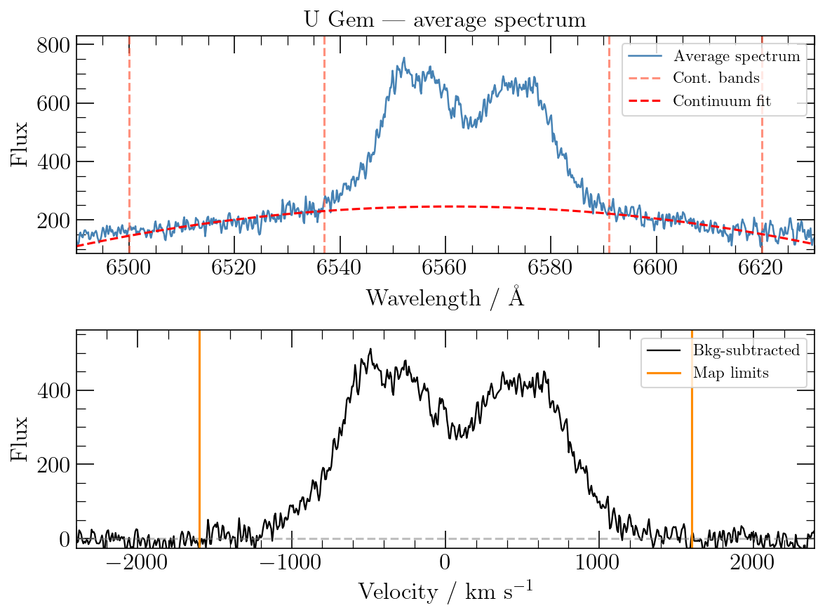
You need to define a continuum band on each side of the emission line, which is used to fit and subtract the continuum.
# Normalise the spectra
dop.Dopin(continnum_band=[6500, 6537, 6591, 6620],
          plot_median=False, poly_degree=2)
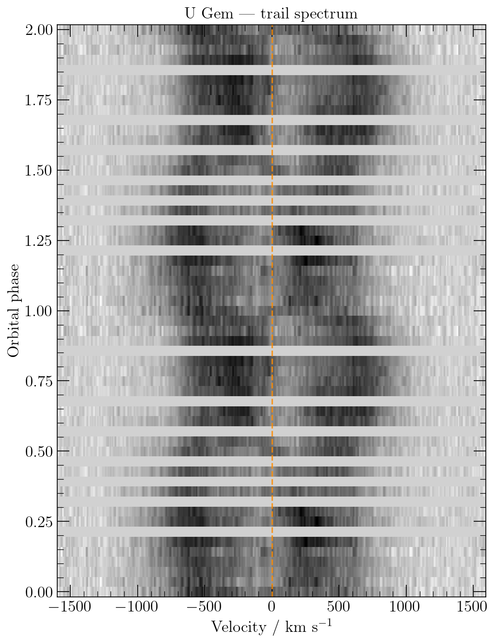
This saves Average_Spec.png (the average spectrum, continuum fit and the
velocity window of the map) and Trail.png (the trail spectrum).
Section 3.3: Run the Doppler tomography
The maximum-entropy reconstruction runs in Python.
# Perform tomography
dop.Syncdop()
Syncdop — MEM Doppler tomography  (native Python)
────────────────────────────────────────────────────────────
→  Map grid:    144 × 144 pixels
→  Input data:  28 phases × 477 velocity channels
→  Projection matrix: sparse, ~29 MB

Alpha step           α     nit         χ    target
──────────  ──────────  ──────  ────────  ────────
✓  α=2.00e-03  nit=  28  χ=1.5233  (target ≤ 1.60)

✓  Converged!  χ = 1.5233  (target ≤ 1.60)  [0.7 s]
→  Final α = 2.00e-03   iterations = 28
→  Entropy S = -2.5016e+04
The map size is set automatically from dop.overs. Pass nv= to
Syncdop() to choose it yourself (e.g. dop.Syncdop(nv=100)).
Section 3.4: Plot the tomography map
This routine displays the result of the Doppler tomography. You can overplot contours and streams.
# Read and plot the map (defaults: linear stretch, magma_r colour map)
fig, data = dop.Dopmap(colorbar=True)

# Overplot the donor contours, keplerian and ballistic streams
qm = 0.35             # mass ratio M_2 / M_1
k1 = 107              # semi-amplitude of the primary in km/s
inc = 70              # inclination angle, in degrees
m1 = 1.2              # mass of the primary in solar masses
porb = 0.1769061911   # orbital period in days

pydoppler.stream(qm, k1, porb, m1, inc,
                 tidal_radius=True, resonance_32=True, resonance_21=True)
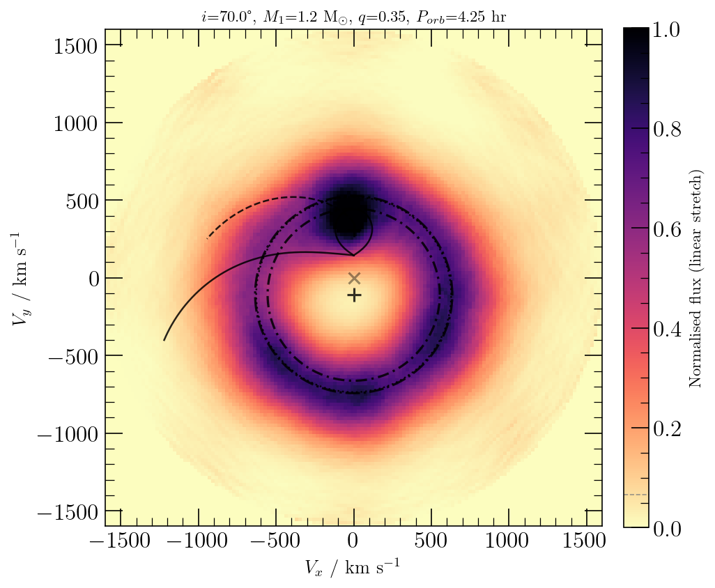
Useful Dopmap options: stretch='linear' | 'sqrt' | 'log',
cmaps=plt.cm.afmhot (or any matplotlib colour map), limits=[lo, hi],
percentile_lo / percentile_hi and smooth=True. With dark colour maps,
pass colors='white' to stream().
Section 3.5: Spectra reconstruction
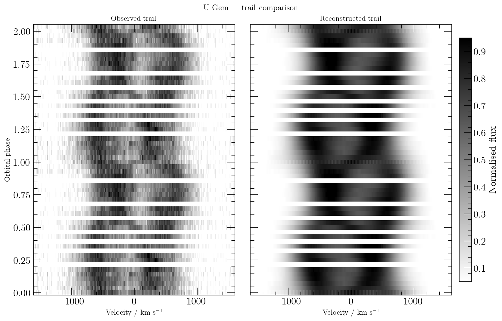
Always check that the reconstructed spectra look like the original ones. A good rule of thumb: "If a feature on the Doppler tomogram is not in the trail spectrum, most likely it's not real!"
# Plot the observed and reconstructed trail spectra
fig, dm, dmr = dop.Reco(colorbar=True, limits=[0.05, 0.95])
Here fig is the figure, and dm and dmr hold the input and reconstructed
trail spectra (phase × velocity, baseline removed), respectively.
Section 4: Extra commands
Many other parameters control the Doppler tomogram. As usual, you can set
them on the pydoppler.spruit object, as in Section 3. The configurable
parameters are:
dop.ih = 0            # type of likelihood function (ih=1 for chi-squared)
dop.iw = 0            # iw=1 if error bars are to be read and used
dop.pb0 = 0.95        # range of phases to be ignored, between 0 and 1
dop.pb1 = 1.05        # range of phases to be ignored, between 1 and 2
dop.ns = 7            # smearing width in default map
dop.ac = 8e-4         # accuracy of convergence
dop.nim = 150         # max no of iterations
dop.al0 = 0.002       # starting value of alpha
dop.alf = 1.7         # factor between successive alphas
dop.nal = 0           # max number of alphas (0 = single alpha)
dop.clim = 1.6        # 'C-aim', target reduced chi
dop.norm = 1          # norm=1 for normalisation to a flat light curve
dop.overs = 0.3       # map oversampling (sets the map size)
What's new in version 1.0
- No Fortran. The Fortran
dop.fengine and themake/gfortranstep are replaced bypydoppler/mem_engine.py, a NumPy/SciPy implementation of the same algorithm (Lucy-accelerated Richardson-Lucy iteration with a floating-default maximum-entropy regularisation). - Fast. The projection matrix is built in vectorised form and stored as a sparse matrix. On the U Gem dataset, the tomography step takes about 0.7 s and the complete sample script about 5 s.
- Checked against Spruit's
dop.f. The projection geometry, default-map smoothing, entropy and its derivatives, baseline handling and alpha schedule follow the Fortran routines (prom,chimg,entr,lamun,basel,alfs). A point-source test recovers the line-of-sight velocities to 0.000 km/s, with no velocity-channel offset. - Safer alpha schedule. When the fit stops improving (at the noise floor of the data), the alpha sequence falls back to geometric steps instead of diverging.
- Plots. New defaults (linear stretch,
magma_r), phases increase upwards in the reconstruction plot, and all routines save their figures.
Development notes
Version 1.0, including the conversion from Fortran to native Python, the
performance optimisation and the line-by-line validation against Spruit's
dop.f, was developed with the help of Claude, Anthropic's AI assistant,
using Claude Opus 5.5 (model claude-opus-5-5) in Claude Code.
Section 5: Troubleshoot
If you find a bug or need a feature, I will try my best to work it out. If you think you can add to this package, I encourage you to push new changes and contribute to it.
1 maintainer

Metadata
1 maintainer
Release files for pydoppler 1.0.0
For a detailed explanation of source distributions (sdists) and built distributions (wheels), please see the package formats documentation.
Source distribution (sdist)
| File | Size | Uploaded | Provenance | Actions |
|---|---|---|---|---|
| pydoppler-1.0.0.tar.gz | 746.0 kB | Without provenance | Details for pydoppler-1.0.0.tar.gz |
Built distribution (wheel)
| File | Interpreter | ABI | Platform | Actions Reset |
|---|---|---|---|---|
| pydoppler-1.0.0-py3-none-any.whl | Python 3 | none | any | Details for pydoppler-1.0.0-py3-none-any.whl |
Total release size: 1.5 MB
Release files / pydoppler-1.0.0.tar.gz
| Download URL | pydoppler-1.0.0.tar.gz |
|---|---|
| Size | 746.0 kB |
| Tags | Source |
|
SHA-256 checksum How to use checksums |
d37194d4dc3da696a41b7dbd36ff4ccddaa224a49690288720e09a693ca82a9d
|
|
BLAKE2b-256 checksum How to use checksums |
31b14f18d9a063e85e3d5a353b9a1e6b526186699e9c4dc17f387ddad0d4f24d
|
| Upload date | |
|
Uploaded using Trusted Publishing? What is trusted publishing? |
No |
| Uploaded via |
twine/6.2.0 CPython/3.9.18
|
Release files / pydoppler-1.0.0-py3-none-any.whl
| Download URL | pydoppler-1.0.0-py3-none-any.whl |
|---|---|
| Size | 756.5 kB |
| Tags | Python 3 |
|
SHA-256 checksum How to use checksums |
d514b76afd736dff9be7dfa2955f687ef5eafd520bf7cf699855b6b406befe9d
|
|
BLAKE2b-256 checksum How to use checksums |
b36b103bb4e7b33c777f99c8070b6b6060943a64397bd75ffcb0d15b9dc759f2
|
| Upload date | |
|
Uploaded using Trusted Publishing? What is trusted publishing? |
No |
| Uploaded via |
twine/6.2.0 CPython/3.9.18
|
Security for pydoppler 1.0.0
Provenance
Provenance describes where a file came from. On PyPI, provenance is shared via attestations, which provide a verifiable record of the build or publishing details. View details, limitations and caveats.
No provenance found
None of the files in this release were uploaded with provenance metadata.
A note on package security
PyPI is a repository for distributing packages, not a service for auditing them. While third-party security researchers and our staff do their best to detect and remove malicious packages, PyPI cannot guarantee the quality, security or suitability of any given package.
To learn more about protecting yourself from malicious actors, visit our package security documentation.














