Ethnobiological data assessment tool.

Project description
pyethnobiology
Ethnobiological data assessment tool
Introduction
This tool is designed to help researchers analyze their ethnobiological data. It is based on the ethnobotanyR package with some modifications. Also, for further information on the methods used in this tool, please refer to the ethnobotanyR package.
Scientific explanations of the indices used in this tool can be found in the documentation of the ethnobotanyR package.
Installation
To install this package, you can use the following code:
pip install pyethnobiology
We recommend use virtualenv to install this package.
Getting started
Importing the package
import pandas as pd
from pyethnobiology import pyethnobiology
Accepted data formats
This package accepts data in the following formats:
- A data frame with the following columns: informant, taxon, uses. The use columns must be binary (0 or 1). For example:
| informant | sp_name | Use_1 | Use_2 | Use_3 | Use_4 | Use_5 |
|---|---|---|---|---|---|---|
| inform_a | sp_a | 0 | 0 | 0 | 1 | 1 |
| inform_a | sp_b | 0 | 0 | 0 | 0 | 0 |
| inform_a | sp_c | 0 | 0 | 1 | 0 | 0 |
| inform_a | sp_d | 0 | 0 | 0 | 0 | 0 |
| inform_b | sp_a | 0 | 1 | 0 | 0 | 1 |
- A data frame with the following columns: informant, taxon, use. The use column must be a string. For example:
| informant | sp_name | ailments_treated |
|---|---|---|
| inform_a | sp_a | Use_3 |
| inform_a | sp_a | Use_8 |
| inform_a | sp_a | Use_9 |
| inform_a | sp_c | Use_6 |
| inform_a | sp_c | Use_7 |
| inform_b | sp_d | Use_3 |
| inform_b | sp_d | Use_6 |
| inform_b | sp_d | Use_7 |
| inform_b | sp_d | Use_8 |
- Literature data is optional for Jaccard index calculation. If there is a multiple literatures, they must be separated by a semicolon. For example:
| informant | sp_name | ailments_treated | literature |
|---|---|---|---|
| inform_a | sp_a | Use_3 | 1 |
| inform_a | sp_a | Use_8 | 1;2 |
| inform_a | sp_a | Use_9 | 1;3;5 |
| inform_a | sp_c | Use_6 | 2 |
| inform_a | sp_c | Use_7 | 1;7 |
| inform_b | sp_d | Use_3 | 3 |
To use this package, you can use the following code:
Load data from csv, excel or txt file
# You can define your separator, for example: sep=";" or sep="\t". By default, the separator is ",".

data = pd.read_csv("{path}/data.csv") # or pd.read_excel("data.xlsx") or pd.read_csv("data.txt")
Load rda (R Data) file
data = "{path}/data.rda"
Define the columns
If uses are binary values in your data (first example in accepted data formats), you don't need to define the use column. But if uses are strings (second example in accepted data formats), you have to define the use column. For example:
# if uses are binary values

informant_column = "informant"
taxon_column = "sp_name"
convert_use_data = True
# if uses are strings

informant_column = "informant"
taxon_column = "sp_name"
use_column = "ailments_treated"
# if you have literature data

informant_column = "informant"
taxon_column = "sp_name"
use_column = "ailments_treated"
literature_column = "literature"
Create an instance of the class
pye = pyethnobiology(data, informant_column, taxon_column, convert_use_data)
You can also define the use column and literature column in the class instance. For example:
pye = pyethnobiology(data, informant_column="informant", taxon_column="sp_name", use_column="ailments_treated")
Indice calculations
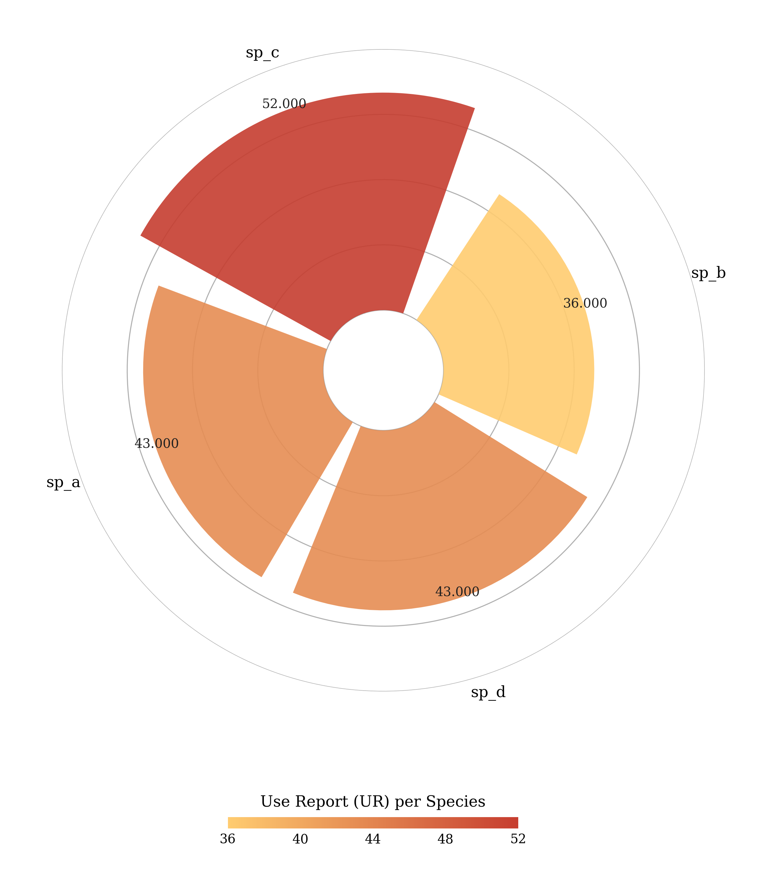
Use Report (UR) per species
pye.UR().calculate()

Out[1]:
  sp_name  UR
0    sp_c  52
1    sp_a  43
2    sp_d  43
3    sp_b  36
Cultural Importance (CI) index
pye.CI().calculate()

Out[1]:
  sp_name  CI
0    sp_c  2.60
1    sp_a  2.15
2    sp_d  2.15
3    sp_b  1.80
Frequency of Citation (FC) per species
pye.FC().calculate()

Out[1]:
  sp_name  FC
0    sp_c  17
1    sp_a  15
2    sp_b  12
3    sp_d  12
Number of Uses (NU) per species
pye.NU().calculate()

Out[1]:
  sp_name  NU
0    sp_c   8
1    sp_d   8
2    sp_a   7
3    sp_b   7
Relative Frequency of Citation (RFC) index
pye.RFC().calculate()

Out[1]:
  sp_name   RFC
0    sp_c  0.85
1    sp_a  0.75
2    sp_b  0.60
3    sp_d  0.60
Relative Importance (RI) index
pye.RI().calculate()

Out[1]:
  sp_name  RI
0    sp_c  1.000000
1    sp_a  0.878676
2    sp_d  0.852941
3    sp_b  0.790441
Use Value (UV) index
pye.UV().calculate()

Out[1]:
  sp_name    UV
0    sp_c  2.60
1    sp_a  2.15
2    sp_d  2.15
3    sp_b  1.80
Cultural Value (CV) for ethnospecies
pye.CV().calculate()

Out[1]:
  sp_name       CV
0    sp_c  1.76800
2    sp_a  1.12875
1    sp_d  1.03200
3    sp_b  0.75600
Fidelity Level (FL) per species
pye.FL().calculate()

Out[1]:
sp_name    ailments_treated         FL
1     sp_a           Use_10  20.000000
2     sp_a            Use_2  53.333333
3     sp_a            Use_3  60.000000
5     sp_a            Use_5  33.333333
6     sp_a            Use_6  46.666667
8     sp_a            Use_8  40.000000
9     sp_a            Use_9  33.333333
10    sp_b            Use_1  50.000000
13    sp_b            Use_3  41.666667
14    sp_b            Use_4  33.333333
15    sp_b            Use_5  33.333333
16    sp_b            Use_6  41.666667
17    sp_b            Use_7  58.333333
19    sp_b            Use_9  41.666667
20    sp_c            Use_1  52.941176
21    sp_c           Use_10  35.294118
22    sp_c            Use_2  41.176471
24    sp_c            Use_4  35.294118
25    sp_c            Use_5  17.647059
26    sp_c            Use_6  23.529412
27    sp_c            Use_7  29.411765
28    sp_c            Use_8  70.588235
30    sp_d            Use_1  41.666667
32    sp_d            Use_2  25.000000
33    sp_d            Use_3  58.333333
35    sp_d            Use_5   8.333333
36    sp_d            Use_6  41.666667
37    sp_d            Use_7  66.666667
38    sp_d            Use_8  75.000000
39    sp_d            Use_9  41.666667
Informant Consensus Factor (FIC)
Informant Consensus Factor (FIC) operates like a consensus barometer, assessing the agreement among individuals. It boils down to a simple equation:

where Nur is the number of use reports for a particular use category and Nt is the number of taxa used for that category. The FIC ranges from 0 to 1, with 0 indicating no agreement among informants and 1 indicating that all informants agree on the taxa to be used for a particular category (Heinrich et al., 1998; Güzel et al., 2015).
pye.FIC().calculate()

Out[1]:
  ailments_treated       FIC
0            Use_8  0.923077
1            Use_3  0.900000
2            Use_7  0.894737
3            Use_1  0.894737
4            Use_4  0.888889
5            Use_2  0.882353
6           Use_10  0.875000
7            Use_9  0.857143
8            Use_6  0.850000
9            Use_5  0.750000
Jaccard similarity index
Jaccard similarity index is a measure of similarity between two sets of data. The higher the Jaccard index, the more similar the two samples are. You can calculate the Jaccard index for all studies or for each study. For example:
pye.jaccard()

Out[1]:
  study  similarity
0     2    0.480000
1     3    0.480000
2     5    0.480000
3     6    0.440000
4     1    0.400000
5     4    0.360000
6     7    0.360000
7     9    0.200000
8    10    0.035714
9     8    0.000000
Mean similarity of all studies:
pye.jaccard()['similarity'].mean()

Out[1]:
    0.32357142857142857

# Round to 2 decimal places
pye.jaccard()['similarity'].mean().round(2)

Out[1]:
    0.32
Visualization
Radial plot
You can plot all indices in a radial plot except Fidelity Level (FL). For example:
#Use Report (UR) per species
pye.UR().plot_radial()
Customization of the radial plot
You can customize the radial plot. For example:
#Use Report (UR) per species
pye.UR().plot_radial(filename="UR.png", # You can define the saving filename. It is default to "UR.png" for UR index.
                     dpi=300, # You can define the dpi. It is default to 300.
                     num_row=10, # It is default to 10 which is the first 10 rows of the data.
                     ytick_position="onbar", # You can define the ytick position. It is default to "onbar".
                     colors=None, # You can define the colors. It is default to None.
                     show_colorbar=True # You can define if you want to show the colorbar. It is default to True.
                     )
num_row means the number of species you want to plot. For example, if you want to plot the first 5 species of the data, you can use the following code:
#Use Report (UR) per species
pye.UR().plot_radial(num_row=5)
You can change the colors of the radial plot. It takes the range of two colors. For example:
#Use Report (UR) per species
pye.UR().plot_radial(colors=["#ECF4D6", "#265073"]) # [minimum value color, maximum value color]

You can also use multiple configurations. For example:
#Use Report (UR) per species
pye.UR().plot_radial(filename="UR_conf.png",
                     dpi=300,
                     num_row=5,
                     ytick_position="onbar", # on_line
                     colors=["#ECF4D6", "#265073"],
                     show_colorbar=False
                     )

Heatmap
You can only plot the Fidelity Level (FL) index in a heatmap. For example:
#Fidelity Level (FL) per species
pye.FL().plot_heatmap()

Customization of the heatmap
You can customize the heatmap. For example:
#Fidelity Level (FL) per species
pye.FL().plot_heatmap(
                     filename="FL.png", # You can define the saving filename. It is default to "FL.png"
                     cmap="coolwarm", # You can define the cmap. It is default to "coolwarm".
                     show_colorbar=True, # You can define if you want to show the colorbar. It is default to True.
                     colorbar_shrink=0.50, # You can define the colorbar shrink. It is default to 0.50.
                     plot_width=10, # You can define the plot width. It is default to 10.
                     plot_height=8, # You can define the plot height. It is default to 8.
                     dpi=300, # You can define the dpi. It is default to 300.
                     fillna_zero=True # You can define if you want to fill the NaN values with 0. It is default to True.
                     )
)
Supported cmaps: https://matplotlib.org/stable/tutorials/colors/colormaps.html
#Fidelity Level (FL) per species
pye.FL().plot_heatmap(filename="FL_reds.png",cmap="Reds")

Chord plot
You can plot all data with the Chord plot. It is diagram of ethnobiological uses and species. For example:
pye.plot_chord()

Customization of the Chord plot
You can customize the Chord plot. For example:
pye.plot_chord(filename="chord_plot.png", # You can define the saving filename. It is default to "chord_plot.png"
               dpi=300, # You can define the dpi. It is default to 300.
               by="taxon", # You can define the by. It is default to "taxon". Other option is "informant".
               colors=None, # You can define the colors. It is default to None.
               min_info_count=0, # You can define the minimum information count for filter data. It is default to 0.
               get_first=None # You can define the number of first data. It is default to None.
               )
You can change the colors of the Chord plot. Supported cmaps: https://matplotlib.org/stable/tutorials/colors/colormaps.html
pye.plot_chord(colors="Dark2")

You can also use multiple configurations. For example:
pye.plot_chord(filename="chord_plot_conf.png",
               dpi=300,
               by="informant",
               colors="tab20b",
               min_info_count=5,
               get_first=10
               )

Release history Release notifications | RSS feed

Download files
Download the file for your platform. If you're not sure which to choose, learn more about installing packages.
Source Distribution
Built Distribution
Filter files by name, interpreter, ABI, and platform.
If you're not sure about the file name format, learn more about wheel file names.
Copy a direct link to the current filters
File details
Details for the file pyethnobiology-0.1.1.tar.gz.
File metadata
- Download URL: pyethnobiology-0.1.1.tar.gz
- Upload date:
- Size: 16.2 kB
- Tags: Source
- Uploaded using Trusted Publishing? No
- Uploaded via: twine/4.0.2 CPython/3.10.9
File hashes
| Algorithm | Hash digest | |
|---|---|---|
| SHA256 |
d5b54d508daa26aeab678a30da1808994c6c37fb53c304e2422e5d414b5f5379
|
|
| MD5 |
c1b59c185f1469c74c7aff6f5f603f45
|
|
| BLAKE2b-256 |
2bbdca691d307c1088db6168b63b1fc31e650f6e31b33df0c29420c66b5a7d68
|
File details
Details for the file pyethnobiology-0.1.1-py3-none-any.whl.
File metadata
- Download URL: pyethnobiology-0.1.1-py3-none-any.whl
- Upload date:
- Size: 17.1 kB
- Tags: Python 3
- Uploaded using Trusted Publishing? No
- Uploaded via: twine/4.0.2 CPython/3.10.9
File hashes
| Algorithm | Hash digest | |
|---|---|---|
| SHA256 |
8e5a9ea38ac5f07741c7c170ab91819d21c2e7ca1c76fadc33c3eef80dd2479f
|
|
| MD5 |
49197a2a41111170b8a4e36ef10368e4
|
|
| BLAKE2b-256 |
b11bbd1ef9c259db1431806313fe1949c877e19e9cd3b5e4b915d4cfdec530ea
|


