
Documentation: https://pygauss.readthedocs.org
Conda Distro: https://binstar.org/cjs14/pygauss
Project: https://github.com/chrisjsewell/PyGauss


PyGauss is intended as an interactive tool for supporting the lifecycle of a computational molecular chemistry investigation. From visual and analytical exploration, through to documentation and publication.
Intitally PyGauss has been designed for the purpose of examining one or more Gaussian quantum chemical computations, both geometrically and electronically. It is built on top of the cclib/chemview/chemlab suite of packages and python scientific stack though, and so should be extensible to other types of computational chemical analysis. PyGauss is primarily designed to be used interactively in the IPython Notebook.
As shown in the examples, a molecular optimisation can be assesed individually (much like in gaussview), but also as part of a group. The advantages of this package are then:
Faster, more efficient analysis
Extensible analysis
Reproducible analysis
Quick Start
OSX and Linux
The recommended was to use pygauss is to download the Anaconda Scientific Python Distribution (64-bit). Once downloaded a new environment can be created in terminal and pygauss installed:
conda create -n pg_env -c https://conda.binstar.org/cjs14 pygauss
Windows
There is currently no pygauss conda distributable for Windows or for chemlab, which has C-extensions that need to be built using a compiler. Please see the documentation for guidance.
Example Assessment
After installing PyGauss you should be able to open this IPython Notebook from; https://github.com/chrisjsewell/PyGauss/blob/master/Example_Assessment.ipynb, and run the following…
from IPython.display import display, Image
%matplotlib inline
import pygauss as pg
print 'pygauss version: {}'.format(pg.__version__)
pygauss version: 0.6.0
The test folder has a number of example Gaussian outputs to play around with.
folder = pg.get_test_folder()
len(folder.list_files())
33
Note: the folder object will act identical whether using a local path or one on a server over ssh (using paramiko):
folder = pg.Folder('/path/to/folder',
                ssh_server='login.server.com',
                ssh_username='username')
Single Molecule Analysis
A molecule can be created containg data about the inital geometry, optimisation process and analysis of the final configuration.
mol = pg.molecule.Molecule(folder_obj=folder,
                init_fname='CJS1_emim-cl_B_init.com',
                opt_fname=['CJS1_emim-cl_B_6-311+g-d-p-_gd3bj_opt-modredundant_difrz.log',
                           'CJS1_emim-cl_B_6-311+g-d-p-_gd3bj_opt-modredundant_difrz_err.log',
                           'CJS1_emim-cl_B_6-311+g-d-p-_gd3bj_opt-modredundant_unfrz.log'],
                freq_fname='CJS1_emim-cl_B_6-311+g-d-p-_gd3bj_freq_unfrz.log',
                nbo_fname='CJS1_emim-cl_B_6-311+g-d-p-_gd3bj_pop-nbo-full-_unfrz.log',
                atom_groups={'emim':range(20), 'cl':[20]},
                alignto=[3,2,1])
Geometric Analysis
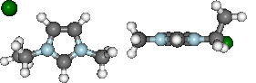
Molecules can be viewed statically or interactively.
#mol.show_initial(active=True)
vdw = mol.show_initial(represent='vdw', rotations=[[0,0,90], [-90, 90, 0]])
ball_stick = mol.show_optimisation(represent='ball_stick', rotations=[[0,0,90], [-90, 90, 0]])
display(vdw, ball_stick)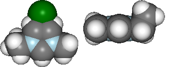
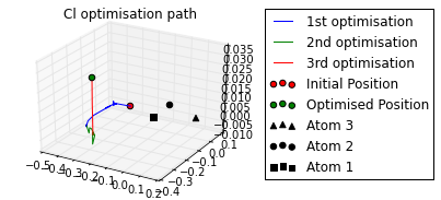
print 'Cl optimised polar coords from aromatic ring : ({0}, {1},{2})'.format(
    *[round(i, 2) for i in mol.calc_polar_coords_from_plane(20,3,2,1)])
ax = mol.plot_opt_trajectory(20, [3,2,1])
ax.set_title('Cl optimisation path')
ax.get_figure().set_size_inches(4, 3)
Cl optimised polar coords from aromatic ring : (0.11, -116.42,-170.06)
Energetics and Frequency Analysis
print('Optimised? {0}, Conformer? {1}, Energy = {2} a.u.'.format(
    mol.is_optimised(), mol.is_conformer(),
    round(mol.get_opt_energy(units='hartree'),3)))
ax = mol.plot_opt_energy(units='hartree')
ax.get_figure().set_size_inches(3, 2)
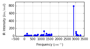
ax = mol.plot_freq_analysis()
ax.get_figure().set_size_inches(4, 2)
Optimised? True, Conformer? True, Energy = -805.105 a.u.

Potential Energy Scan analysis of geometric conformers…
mol2 = pg.molecule.Molecule(folder_obj=folder, alignto=[3,2,1],
            pes_fname=['CJS_emim_6311_plus_d3_scan.log',
                       'CJS_emim_6311_plus_d3_scan_bck.log'])
ax = mol2.plot_pes_scans([1,4,9,10], rotation=[0,0,90], img_pos='local_maxs', zoom=0.5)
ax.set_title('Ethyl chain rotational conformer analysis')
ax.get_figure().set_size_inches(7, 3)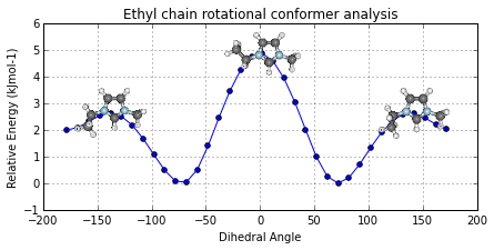
Partial Charge Analysis
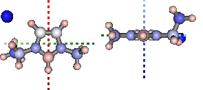
using Natural Bond Orbital (NBO) analysis
print '+ve charge centre polar coords from aromatic ring: ({0} {1},{2})'.format(
    *[round(i, 2) for i in mol.calc_nbo_charge_center(3, 2, 1)])
display(mol.show_nbo_charges(represent='ball_stick', axis_length=0.4,
                              rotations=[[0,0,90], [-90, 90, 0]]))
+ve charge centre polar coords from aromatic ring: (0.02 -51.77,-33.15)
Density of States Analysis
print 'Number of Orbitals: {}'.format(mol.get_orbital_count())
homo, lumo = mol.get_orbital_homo_lumo()
homoe, lumoe = mol.get_orbital_energies([homo, lumo])
print 'HOMO at {} eV'.format(homoe)
print 'LUMO at {} eV'.format(lumoe)
Number of Orbitals: 272 HOMO at -4.91492036773 eV LUMO at -1.85989816817 eV
ax = mol.plot_dos(per_energy=1, lbound=-20, ubound=10, legend_size=12)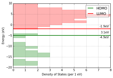
Bonding Analysis
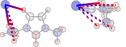
Using Second Order Perturbation Theory.
print 'H inter-bond energy = {} kJmol-1'.format(
        mol.calc_hbond_energy(eunits='kJmol-1', atom_groups=['emim', 'cl']))
print 'Other inter-bond energy = {} kJmol-1'.format(
    mol.calc_sopt_energy(eunits='kJmol-1', no_hbonds=True, atom_groups=['emim', 'cl']))
display(mol.show_sopt_bonds(min_energy=1, eunits='kJmol-1',
                            atom_groups=['emim', 'cl'],
                            no_hbonds=True,
                            rotations=[[0, 0, 90]]))
display(mol.show_hbond_analysis(cutoff_energy=5.,alpha=0.6,
                                atom_groups=['emim', 'cl'],
                                rotations=[[0, 0, 90], [90, 0, 0]]))
H inter-bond energy = 111.7128 kJmol-1 Other inter-bond energy = 11.00392 kJmol-1

Multiple Computations Analysis
Multiple computations, for instance of different starting conformations, can be grouped into an Analysis class and anlaysed collectively.
analysis = pg.Analysis(folder_obj=folder)
errors = analysis.add_runs(headers=['Cation', 'Anion', 'Initial'],
                               values=[['emim'], ['cl'],
                                       ['B', 'BE', 'BM', 'F', 'FE']],
            init_pattern='*{0}-{1}_{2}_init.com',
            opt_pattern='*{0}-{1}_{2}_6-311+g-d-p-_gd3bj_opt*unfrz.log',
            freq_pattern='*{0}-{1}_{2}_6-311+g-d-p-_gd3bj_freq*.log',
            nbo_pattern='*{0}-{1}_{2}_6-311+g-d-p-_gd3bj_pop-nbo-full-*.log',
            alignto=[3,2,1], atom_groups={'emim':range(1,20), 'cl':[20]},
            ipython_print=True)
Reading data 5 of 5
Molecular Comparison
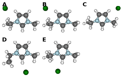
fig, caption = analysis.plot_mol_images(mtype='optimised', max_cols=3,
                        info_columns=['Cation', 'Anion', 'Initial'],
                        rotations=[[0,0,90]])
print caption
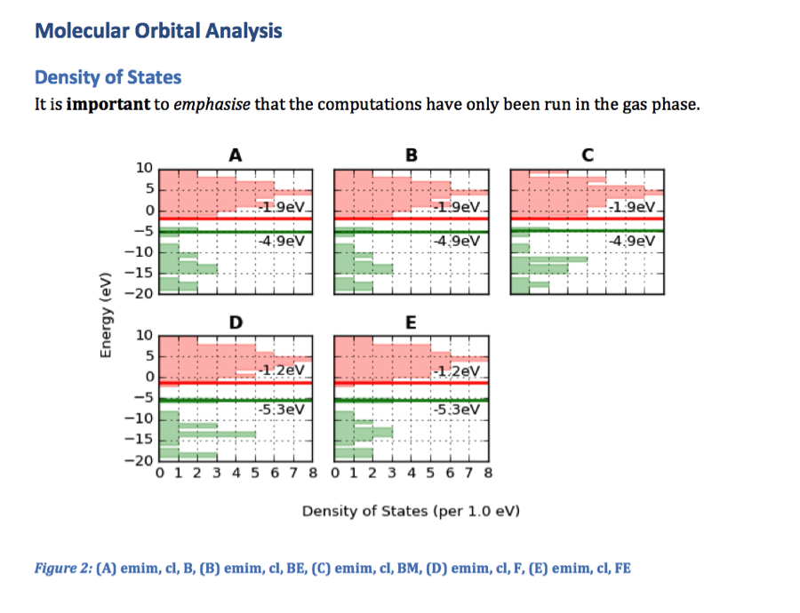
(A) emim, cl, B, (B) emim, cl, BE, (C) emim, cl, BM, (D) emim, cl, F, (E) emim, cl, FE
Data Comparison
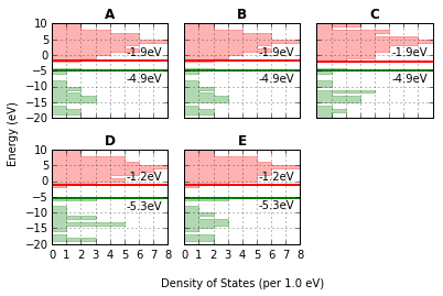
fig, caption = analysis.plot_mol_graphs(gtype='dos', max_cols=3,
                                        lbound=-20, ubound=10, legend_size=0,
                                        band_gap_value=False,
                                   info_columns=['Cation', 'Anion', 'Initial'])
print caption
(A) emim, cl, B, (B) emim, cl, BE, (C) emim, cl, BM, (D) emim, cl, F, (E) emim, cl, FE
The methods mentioned for indivdiual molecules can be applied to all or a subset of these computations.
analysis.add_mol_property_subset('Opt', 'is_optimised', rows=[2,3])
analysis.add_mol_property('Energy (au)', 'get_opt_energy', units='hartree')
analysis.add_mol_property('Cation chain, $\\psi$', 'calc_dihedral_angle', [1, 4, 9, 10])
analysis.add_mol_property('Cation Charge', 'calc_nbo_charge', 'emim')
analysis.add_mol_property('Anion Charge', 'calc_nbo_charge', 'cl')
analysis.add_mol_property(['Anion-Cation, $r$', 'Anion-Cation, $\\theta$', 'Anion-Cation, $\\phi$'],
                               'calc_polar_coords_from_plane', 3, 2, 1, 20)
analysis.add_mol_property('Anion-Cation h-bond', 'calc_hbond_energy',
                          eunits='kJmol-1', atom_groups=['emim', 'cl'])
analysis.get_table(row_index=['Anion', 'Cation', 'Initial'],
                   column_index=['Cation', 'Anion', 'Anion-Cation'])
There is also an option (requiring pdflatex and ghostscript+imagemagik) to output the tables as a latex formatted image.
analysis.get_table(row_index=['Anion', 'Cation', 'Initial'],
                   column_index=['Cation', 'Anion', 'Anion-Cation'],
                   as_image=True, font_size=12)
Multi-Variate Analysis
RadViz is a way of visualizing multi-variate data.
ax = analysis.plot_radviz_comparison('Anion', columns=range(4, 10))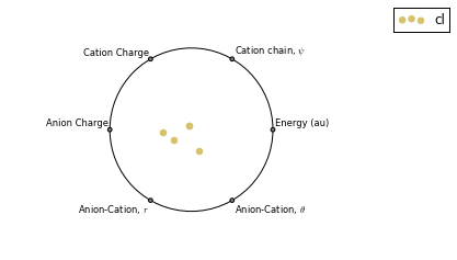
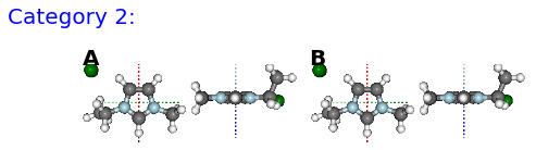
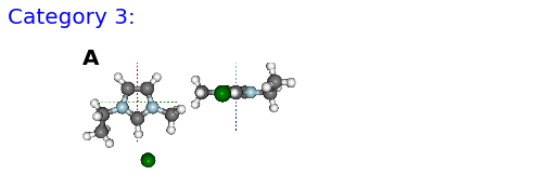
The KMeans algorithm clusters data by trying to separate samples into n groups of equal variance.
pg.utils.imgplot_kmean_groups(
    analysis, 'Anion', 'cl', 4, range(4, 10),
    output=['Initial'], mtype='optimised',
    rotations=[[0, 0, 90], [-90, 90, 0]],
    axis_length=0.3)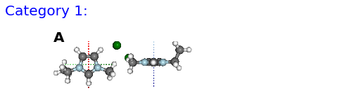
(A) BM
(A) FE
(A) B, (B) BE

(A) F
Documentation (MS Word)
After analysing the computations, it would be reasonable to want to document some of our findings. This can be achieved by outputting individual figure or table images via the folder object.
file_path = folder.save_ipyimg(vdw, 'image_of_molecule')
Image(file_path)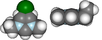
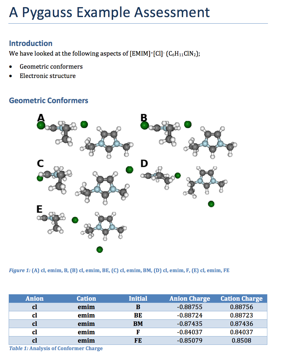
But you may also want to produce a more full record of your analysis, and this is where python-docx steps in. Building on this package the pygauss MSDocument class can produce a full document of your analysis.
import matplotlib.pyplot as plt
d = pg.MSDocument()
d.add_heading('A Pygauss Example Assessment', level=0)

d.add_docstring("""
# Introduction

We have looked at the following aspects
of [EMIM]^{+}[Cl]^{-} (C_{6}H_{11}ClN_{2});

- Geometric conformers
- Electronic structure

# Geometric Conformers
""")

fig, caption = analysis.plot_mol_images(max_cols=2,
                rotations=[[90,0,0], [0,0,90]],
                info_columns=['Anion', 'Cation', 'Initial'])
d.add_mpl(fig, dpi=96, height=9, caption=caption)
plt.close()
d.add_paragraph()
df = analysis.get_table(
        columns=['Anion Charge', 'Cation Charge'],
        row_index=['Anion', 'Cation', 'Initial'])
d.add_dataframe(df, incl_indx=True, style='Medium Shading 1 Accent 1',
                caption='Analysis of Conformer Charge')

d.add_docstring("""
# Molecular Orbital Analysis
## Density of States

It is **important** to *emphasise* that the
computations have only been run in the gas phase.
""")
fig, caption = analysis.plot_mol_graphs(gtype='dos', max_cols=3,
                                    lbound=-20, ubound=10, legend_size=0,
                                    band_gap_value=False,
                               info_columns=['Cation', 'Anion', 'Initial'])
d.add_mpl(fig, dpi=96, height=9, caption=caption)
plt.close()

d.save('exmpl_assess.docx')
Which gives us the following:
MORE TO COME!!
1 maintainer

Release files for pygauss 0.6.0
For a detailed explanation of source distributions (sdists) and built distributions (wheels), please see the package formats documentation.
Source distribution (sdist)
| File | Size | Uploaded | |
|---|---|---|---|
| pygauss-0.6.0.tar.gz | 4.9 MB | Details |
Release files / pygauss-0.6.0.tar.gz
| Download URL | pygauss-0.6.0.tar.gz |
|---|---|
| Size | 4.9 MB |
| Tags | Source |
|
SHA-256 checksum How to use checksums |
9e69d46aa6d2b48937ee45b7c7c9ee63a8ab90b606fa1da6aa60429d81728f28
|
|
BLAKE2b-256 checksum How to use checksums |
c851a6dadab41f89c0c7808b80c01c855d5a3d70a67f47d9894023ebada3c938
|
| Upload date | |
|
Uploaded using Trusted Publishing? What is trusted publishing? |
No |














