
Implementation of an algorithm from the field of global optimization according to the publication ‘The improvement function in branch-and-bound methods for complete global optimization’ by P. Kirst, M. Rodestock, S. Schwarze and O. Stein.

Project description
pyimpBB - A branch-and-bound method using the improvement function in Python
This package provides the implementation of a novel branch-and-bound algorithm for the outer approximation of all global minimal points of a nonlinear constrained optimization problem using the improvement function, internally referred to as 'improved_BandB', to the corresponding publication 'The improvement function in branch-and-bound methods for complete global optimization' by P. Kirst, M. Rodestock, S. Schwarze and O. Stein.
Installation:
The easiest and yet preferred way to install this package is to use pip. This allows you to install the package either directly from PyPi:
python3 -m pip install --upgrade pip
python3 -m pip install pyimpBB
or from a download of the source on PyPi:
python3 -m pip install --upgrade pip
python3 -m pip download pyimpBB
python3 -m pip install *.whl
or github:
python3 -m pip install --upgrade pip setuptools wheel
git clone https://github.com/uisab/Python_Code.git
python3 -m pip setup.py sdist bdist_wheel
python3 -m pip install dist/*.whl
In case of problems with the required packages pyinterval (or crlibm) during installation, try python3 -m pip install 'setuptools<=74.1.3' or look out here.
Structure/ API:
The package consists of the four modules pyimpBB.helper, pyimpBB.bounding, pyimpBB.solver and pyimpBB.analyzing, each of which represents a core task of the implementation and provides Python classes and functions corresponding to their name. The following table gives an overview of these modules and their relevant classes and functions with a short description of each. For more detailed descriptions of the functionality, input and output, use help(<module/class/function name>).
| Modules | Classes/ functions | Description |
|---|---|---|
| helper | class obvec(tuple) | A vector consisting of arbitrary objects with vector-valued support for all elementary operations (+,-,*,/,&,|,...) as well as the scalar product (@). |
| class obmat(tuple) | A matrix consisting of arbitrary objects with matrix-valued support for all elementary operations (+,-,*,/,&,|,...) as well as the matrix product (@). | |
| class intvec(obvec) | A vector consisting of intervals from the pyinterval package, which supports all elementary operations (+,-,*,/,&,|,...) as well as the scalar product (@) interval-valued. | |
| exp(x), log(x), sin(x), cos(x), tan(x), sqrt(x) | Refers to the corresponding mathematical function matching the input type. | |
| bounding | direct_intervalarithmetic(func, grad, hess, X, direction) | Uses pur interval arithmetic to return an upper or lower bound of the real function 'func' on the interval-vector 'X' in the form of an object-vector. |
| centered_forms(func, grad, hess, X, direction) | Uses centered forms to return an upper or lower bound of the real potentially vector-valued function 'func' on the interval-vector 'X' in the form of an object-vector. | |
| optimal_centerd_forms(func, grad, hess, X, direction) | Uses optimal centered forms to return an upper or lower bound of the real function 'func' on the interval-vector 'X' in the form of an object-vector. | |
| aBB_relaxation(func, grad, hess, X, direction) | Uses konvex relaxation via aBB method to return an upper or lower bound of the real function 'func' on the interval-vector 'X' in the form of an object-vector. | |
| solver | improved_BandB(func, cons, X, bounding_procedure, grad=None, hess=None, cons_grad=[], cons_hess=[], epsilon=0, delta=0, epsilon_max=0.5, delta_max=0.5, max_iter=2500) | Uses the improvement function in the course of a branch-and-bound approach to provide an enclosure of the solution set of a nonlinear constrained optimization problem with a given accuracy. |
| analysed_improved_BandB(func, cons, X, bounding_procedure, grad=None, hess=None, cons_grad=[], cons_hess=[], epsilon=0, delta=0, epsilon_max=0.5, delta_max=0.5, search_ratio=0, max_time=60, save_lists=True) | A variation of 'improved_BandB' that provides mixed breadth-depth-first search, a numerically useful second termination condition and collects additional data generally and optionally per iteration to support subsequent analysis of the approximation progress and results. | |
| improved_boxres_BandB(func, X, bounding_procedure, grad=None, hess=None, epsilon=0, epsilon_max=0.5, max_iter=2500) | Uses the improvement function in the course of a branch-and-bound approach to provide an enclosure of the solution set of a nonlinear box-constrained optimization problem with a given accuracy. | |
| analysed_improved_boxres_BandB(func, X, bounding_procedure, grad=None, hess=None, epsilon=0, epsilon_max=0.5, search_ratio=0, max_time=60, save_lists=True) | A variation of 'improved_boxres_BandB' that provides mixed breadth-depth-first search, a numerically useful second termination condition and collects additional data generally and optionally per iteration to support subsequent analysis of the approximation progress and results. | |
| analyzing | iterations_in_decision_space_plot(func, X, data, iterations, cons=None, title="...", subtitle="...", fname=None, columns=3, levels=None, cons_deltas=None, mgres=100, xylim=None, legend_labels=None, **args) | Generates a tabular representation in which the decision space is shown for given iterations, including level lines of the objective function, zero level lines of the constraints, enclosing box X and associated approximation or decomposition progress. |
| iterations_in_objective_space_plot(func, X, data, iterations, grad=None, cons=None, title='...', subtitle="...", fname=None, columns=3, dspace=True, mgres=100, xyzlim=None, legend_labels=None, **args) | Generates a tabular representation in which the objective space is shown for given iterations, including the surface of the objective function, the associated optimal value approximation progress and optionally the decision space. |
Application:
The use of this package will be shown and explained using a simple example. To do this, consider the optimization problem of the form
$$\min_x f(x) \quad s.t. \quad \omega(x) = \max\lbrace \omega_1(x), \ldots, \omega_4(x) \rbrace \leq 0,\quad\negthickspace x \in X$$
with nonempty box $X := ([0,4],[0,4])^\intercal \subseteq \mathbb{I}\negthinspace\mathbb{R}^2$ and continuously differentiable functions $f,\omega_i: \mathbb{R}^2 \rightarrow \mathbb{R}, i \in \lbrace 1, \ldots, 4\rbrace$ defined as
$$f(x) := x_1 + x_2,$$ $$\omega_1(x) := -(x_1^2 + x_2^2) +6.5, \quad \omega_3(x) := x_1 -x_2 -2,$$ $$\omega_2(x) := -x_1 +x_2 -2, \qquad\negthickspace \omega_4(x) := x_1^2 +x_2^2 -16.$$
This example problem should now be solved using the algorithm provided by this package and then analyzed using the representation functions also provided. To do this, it can first be modeled as follows using the class intvec from the module pyimpBB.helper.
from pyimpBB.helper import intvec

X = intvec([[0,4],[0,4]])

def func(x):
    return x[0] + x[1]

def omega_1(x):
    return -(x[0]**2 +x[1]**2) +6.5

def omega_2(x):
    return -x[0] +x[1] -2

def omega_3(x):
    return x[0] -x[1] -2

def omega_4(x):
    return x[0]**2 +x[1]**2 -16
Here, intvec not only provides a simple way of instantiating a vector of intervals, but also some required properties, such as their width width() and splitting split(). As can be seen, it is instantiated using an $n$-element list of lists with exactly two entries, which correspond to the upper and lower bounds of the intervals. The interval objects used in this context come from the pyinterval package and have an interval-valued implementation of all elementary operations (+,-,*,/,&,...). The two classes obvec and obmat from the pyimpBB.helper module are used as follows to model the first and second derivatives that are required later depending on the selected bounding procedure.
from pyimpBB.helper import obvec, obmat

def grad(x):
    return obvec([1,1])
def hess(x):
    return obmat([[0,0],[0,0]])

def omega_1_grad(x):
    return obvec([-2*x[0],-2*x[1]])
def omega_1_hess(x):
    return obmat([[-2,0],[0,-2]])

def omega_2_grad(x):
    return obvec([-1,1])
def omega_2_hess(x):
    return obmat([[0,0],[0,0]])

def omega_3_grad(x):
    return obvec([1,-1])
def omega_3_hess(x):
    return obmat([[0,0],[0,0]])

def omega_4_grad(x):
    return obvec([2*x[0],2*x[1]])
def omega_4_hess(x):
    return obmat([[2,0],[0,2]])
They represent a vector or a matrix of arbitrary Python objects and have a corresponding vector or matrix-valued implementation of all elementary operations (+,-,*,/,&,|,...) as well as the scalar or matrix product (@). In order to ensure the functionality of the required vector-valued interval arithmetic, its use should not be abandoned in favor of better known alternatives, such as numpy.ndarray. However, both support conversion to and from numpy.ndarray, which means that all functions of the numpy package can be used. It should be noted that the instantiation of obmat is done column-wise compared to numpy.ndarray. The following table shows the bounding procedures available in the pyimpBB.bounding module, along with their differentiability requirements.
| Bounding procedures | First derivative/ gradient | Second derivative/ hessian |
|---|---|---|
| direct_intervalarithmetic(func, grad, hess, X, direction) | False | False |
| centered_forms(func, grad, hess, X, direction) | True | False |
| optimal_centerd_forms(func, grad, hess, X, direction) | True | False |
| aBB_relaxation(func, grad, hess, X, direction) | True | True |
In order to be able to apply the algorithm designed for such problems in the form of the function analysed_improved_BandB() from the module pyimpBB.solver with a selected bound operation, such as aBB_relaxation(), it is still necessary to specify certain accuracies with regard to the feasibility (delta, delta_max) and optimality (epsilon, epsilon_max) of the solution as well as to define three auxiliary variables in the form of lists for clear transfer.
from pyimpBB.bounding import aBB_relaxation
from pyimpBB.solver import analysed_improved_BandB

cons = [omega_1,omega_2,omega_3,omega_4]
cons_grad = [omega_1_grad,omega_2_grad,omega_3_grad,omega_4_grad]
cons_hess = [omega_1_hess,omega_2_hess,omega_3_hess,omega_4_hess]

solution, y_best, k, t, save = analysed_improved_BandB(func, cons, X, bounding_procedure=aBB_relaxation, grad=grad, hess=hess, cons_grad=cons_grad, cons_hess=cons_hess)
The return of this function consists of the actual solution of the algorithm as a list of intvec, the best incumbent found during the procedure as an obvec, the number of iterations required as an integer, the time required/elapsed by the algorithm in seconds as a float-value and a dictionary provided for analysis purposes, which documents the approximation progress of the algorithm for each iteration. With the help of the two functions iterations_in_decision_space_plot and iterations_in_objective_space_plot from the module pyimpBB.analyzing this progress can be displayed graphically, with both having an extensive range of options for influencing the resulting graphic. To use these functions, the data to be displayed must be extracted from the return of the function analysed_improved_BandB() as a dictionary with the iterations as keys and a selection of the iterations to be displayed as a list.
from pyimpBB.analyzing import iterations_in_decision_space_plot

data = dict(zip(save.keys(),[[Oi[0] for Oi in save[k][0]] for k in save]))
iterations = list(data.keys())[::round(k/3)]

iterations_in_decision_space_plot(func,X,data,iterations,cons=cons,columns=2,levels=[3,3.5],figsize=(8,6),facecolor="white")
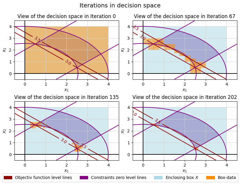
In this plot, the box $X$ (colored light blue), the feasible set $\Omega := \lbrace x \in X \mid \omega(x) \leq 0 \rbrace$ (colored purple), the course of the objective function $f$ based on the level lines to the global minimum value $v$ and $v$ + epsilon_max (red) and the iterative approximation progress of the algorithm (colored orange) are clearly visible. However, since such a graphical view of the results only proves to be useful for two-dimensional problems, the corresponding functions can only be applied to these. At the end of this example, for the theoretical background, reference is made to the already mentioned publication 'The improvement function in branch-and-bound methods for complete global optimization' by P. Kirst, M. Rodestock, S. Schwarze and O. Stein.
Miscellaneous
This package was created as part of a master thesis ('Analysis of a branch-and-bound method for nonlinear constrained optimization problems' by M. Rodestock) and we strive to provide a high-quality presentation to the best of our knowledge and belief. However, the author assumes no responsibility for the use of this package in any context. If you have suggestions for improvement or requests, the author asks for your understanding if he tends not to comply with them in the long term. Otherwise, enjoy this little package!
(written on 14.04.2025)


Download files
Download the file for your platform. If you're not sure which to choose, learn more about installing packages.
Source Distribution
Built Distribution
Filter files by name, interpreter, ABI, and platform.
If you're not sure about the file name format, learn more about wheel file names.
Copy a direct link to the current filters
File details
Details for the file pyimpbb-0.1.0.tar.gz.
File metadata
- Download URL: pyimpbb-0.1.0.tar.gz
- Upload date:
- Size: 21.0 kB
- Tags: Source
- Uploaded using Trusted Publishing? No
- Uploaded via: twine/6.1.0 CPython/3.9.12
File hashes
| Algorithm | Hash digest | |
|---|---|---|
| SHA256 |
d542f41c2df2d197e09bf5c3b7406599b98d0d2bddb278117e5610c2c0ca8d0d
|
|
| MD5 |
2cc9a41fc71afcad0dd835b9da182ac3
|
|
| BLAKE2b-256 |
b5521387bf429fb9fc984ed1f4be99c2d1f594b151d6230f8a758357bcaf8a5e
|
File details
Details for the file pyimpbb-0.1.0-py3-none-any.whl.
File metadata
- Download URL: pyimpbb-0.1.0-py3-none-any.whl
- Upload date:
- Size: 18.2 kB
- Tags: Python 3
- Uploaded using Trusted Publishing? No
- Uploaded via: twine/6.1.0 CPython/3.9.12
File hashes
| Algorithm | Hash digest | |
|---|---|---|
| SHA256 |
3fc1320c0b3d7e3e839d45e0b03f7aa69ad85e926886f0d7938841f977f48e1b
|
|
| MD5 |
769829db79519fb294b6fd21746c2227
|
|
| BLAKE2b-256 |
2cabc1b0ecac83b1ffcd40f6ed3d3b77d71c88c4945ebd295268f3952a008c6c
|






