
Mass ratio variance-based outlier factor (MOF)

Project description
pymof
Updated by Mr. Supakit Sroynam (6534467323@student.chula.ac.th) and Krung Sinapiromsaran (krung.s@chula.ac.th)
Department of Mathematics and Computer Science, Faculty of Science, Chulalongkorn University
Version 0.2: 23 September 2024
Version 0.3: 9 October 2024
Version 0.4: 12 October 2024
Version 0.5: 8 January 2025
Version 0.6: 27 November 2025
Version 0.7: 12 December 2025
Mass-ratio-variance based outlier factor
Latest news
- Implementing HVOF() for detecting anomaly in data stream.
- Documents are editted with more methods.
- A Table of Contents is added.
Introduction
An outlier in a finite dataset is a data point that stands out from the rest. It is often isolaed, unliked normal data points, which tend to cluster together. To identify outliers, the Mass-ratio-variance based Outlier Factor (MOF) was developed and implemented. MOF works by calculating a score of each data point based on the density of itself with respect to other data points. Outliers always have fewer nearby data points so their mass-ratio (a density ratio if the same volumes are used) will be different from normal points. This MOF algorithm does not require any extra settings.
Citation
If you use this package in your research, please consider citing these two papers.
BibTex for the package:
@inproceedings{changsakul2021mass,
  title={Mass-ratio-variance based Outlier Factor},
  author={Changsakul, Phichapop and Boonsiri, Somjai and Sinapiromsaran, Krung},
  booktitle={2021 18th International Joint Conference on Computer Science and Software Engineering (JCSSE)},
  pages={1--5},
  year={2021},
  organization={IEEE}
}
@INPROCEEDINGS{10613697,
  author={Fan, Zehong and Luangsodsai, Arthorn and Sinapiromsaran, Krung},
  booktitle={2024 21st International Joint Conference on Computer Science and Software Engineering (JCSSE)},
  title={Mass-Ratio-Average-Absolute-Deviation Based Outlier Factor for Anomaly Scoring},
  year={2024},
  volume={},
  number={},
  pages={488-493},
  keywords={Industries;Software algorithms;Process control;Quality control;Nearest neighbor methods;Fraud;Computer security;Anomaly scoring;Statistical dispersion;Mass-ratio distribution;Local outlier factor;Mass-ratio variance outlier factor},
  doi={10.1109/JCSSE61278.2024.10613697}}
Installation
To install pymof, type the following command in the terminal
pip install pymof            # normal install
pip install --upgrade pymof  # or update if needed
Use on jupyter notebook
To make sure that the installed package can be called. A user must include the package path before import as
import sys
sys.path.append('/path/to/lib/python3.xx/site-packages')
Required Dependencies :
- Python 3.9 or higher
- numpy>=1.23
- numba>=0.56.0
- scipy>=1.8.0
- scikit-learn>=1.2.0
- matplotlib>=3.5
Documentation
Table of Contents
- Mass-ratio-variance based Outlier Factor (MOF)
- Mass-Ratio-Average-Absolute-Deviation Based Outlier Factor (MAOF)
- Windowing mass-ratio-variance based outlier factor (WMOF)
- Hypervolume-ratio-variance Outlier Factor (HVOF)
Mass-ratio-variance based Outlier Factor (MOF)
The outlier score of each data point is calculated using the Mass-ratio-variance based Outlier Factor (MOF). MOF quantifies the global deviation of a data point's density relative to the rest of the dataset. This global perspective is crucial because an outlier's score depends on its overall isolation from all other data points. By analyzing the variance of the mass ratio, MOF can effectively identify data points with significantly lower density compared to their neighbors, indicating their outlier status.
MOF()
Initialize a model object
MOF
    Parameters :
    Return :
            self : object
                    object of MOF model
MOF.fit(Data, Window = 10000, KeepMassRatio = True)
Fit data to
MOFmodel
    Parameters :
            Data  : numpy array of shape (n_points, d_dimensions)
                    The input samples.
            Window : integer (int)
                    window size for calculation.
                    default window size is 10000.
            KeepMassRatio : boolean
                    All points' mass ratio are kept when an argument is True.
                    Beware of exploding memory since calculation with window size = n.
                    Can be set to False for memory efficient.
                    default KeepMassRatio size is True.
    Return :
            self  : object
                    fitted estimator
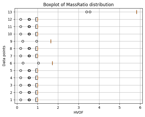
MOF.visualize()
Visualize data points with
MOF's scores
Note cannot visualize data points having a dimension greather than 3
    Parameters :
    Return :
            decision_scores_ : numpy array of shape (n_samples)
                    decision score for each point
MOF attributes
| Attributes | Type | Details |
|---|---|---|
| MOF.Data | numpy array of shape (n_points, d_dimensions) | input data for scoring |
| MOF.decision_scores_ | numpy array of shape (n_samples) | decision score for each point |
| MOF.MassRatio | numpy array of shape (n_samples, n_samples-1) | mass ratio for each pair of points (exclude self pair) |
Sample usage
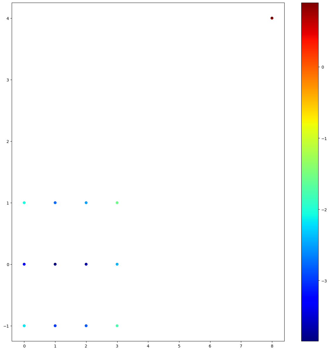
# This example is from MOF paper.
from pymof import MOF
import numpy as np
import matplotlib.pyplot as plt
data = np.array([[0.0, 1.0], [1.0, 1.0], [2.0, 1.0], [3.0, 1.0],
                 [0.0, 0.0], [1.0, 0.0], [2.0, 0.0], [3.0, 0.0],
                 [0.0,-1.0], [1.0,-1.0], [2.0,-1.0], [3.0,-1.0], [8.0, 4.0]
                ])
model = MOF()
model.fit(data)
scores = model.decision_scores_
print(scores)
model.visualize()

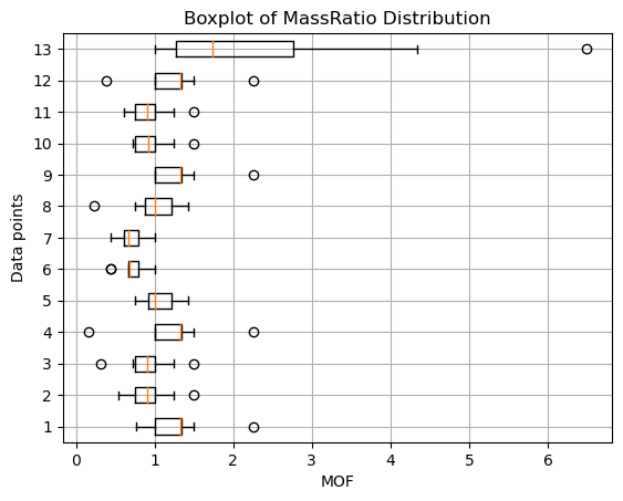
# Create a figure and axes
fig, ax = plt.subplots()
data = model.MassRatio
# Iterate over each row and create a boxplot
for i in range(data.shape[0]):
    row = data[i, :]
    mask = np.isnan(row)
    ax.boxplot(row[~mask], positions=[i + 1], vert=False, widths=0.5)
# Set labels and title
ax.set_xlabel("MOF")
ax.set_ylabel("Data points")
ax.set_title("Boxplot of MassRatio distribution")
# Show the plot
plt.grid(True)
plt.show()
Output
[0.12844997, 0.06254347, 0.08142683, 0.20940997, 0.03981233, 0.0212412 , 0.025438 , 0.08894882, 0.11300615, 0.0500218, 0.05805704, 0.17226989, 2.46193377]
3D sample
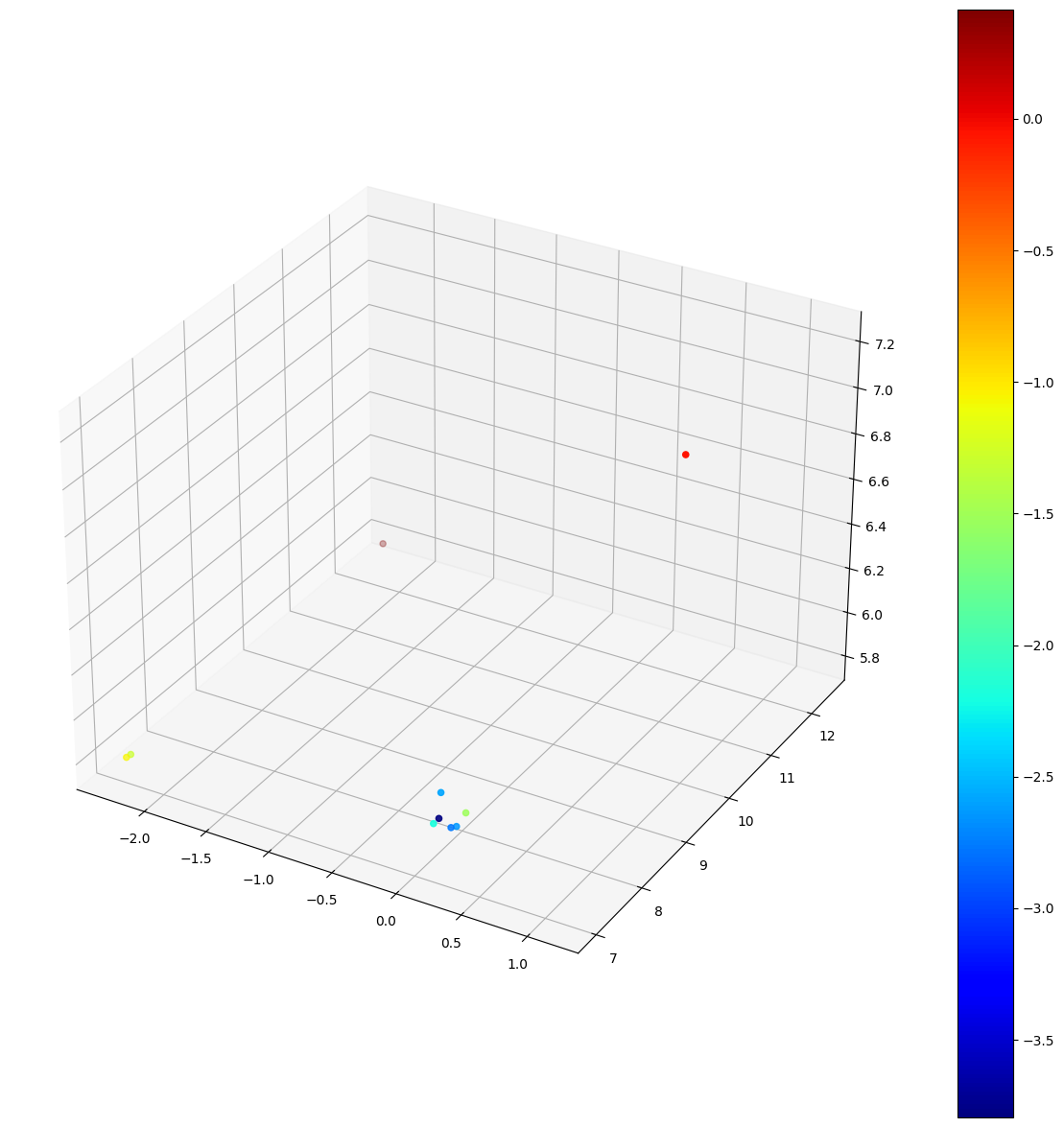
# This example demonstrates  the usage of MOF
import numpy as np
from pymof import MOF
data = np.array([[-2.30258509,  7.01040212,  5.80242044],
                 [ 0.09531018,  7.13894636,  5.91106761],
                 [ 0.09531018,  7.61928251,  5.80242044],
                 [ 0.09531018,  7.29580291,  6.01640103],
                 [-2.30258509, 12.43197678,  5.79331844],
                 [ 1.13140211,  9.53156118,  7.22336862],
                 [-2.30258509,  7.09431783,  5.79939564],
                 [ 0.09531018,  7.50444662,  5.82037962],
                 [ 0.09531018,  7.8184705,   5.82334171],
                 [ 0.09531018,  7.25212482,  5.91106761]])
model = MOF()
model.fit(data)
scores = model.decision_scores_
print(scores)
model.visualize()
Output
[0.34541068 0.11101711 0.07193073 0.07520904 1.51480377 0.94558894 0.27585581 0.06242823 0.2204504 0.02247725]
Mass-Ratio-Average-Absolute-Deviation Based Outlier Factor (MAOF)
Mass-Ratio-Average-Absolute-Deviation Based Outlier Factor for Anomaly Scoring (MAOF) This research extends the mass-ratio-variance outlier factor algorithm (MOF) by exploring other alternative statistical dispersions beyond the traditional variance such as range, interquartile range (IQR), average absolute deviation (AAD), and convex combination of IQR and AAD.
MAOF()
Initialize a model object
MAOF
    Parameters :
    Return :
            self : object
                    object of MAOF model
MAOF.fit(Data, Window = 10000, Function_name = "AAD", Weight_Lambda = 0.5, KeepMassRatio = True)
Fit data to
MAOFmodel
    Parameters :
            Data  : numpy array of shape (n_points, d_dimensions)
                    The input samples.
            Window  : int
                    number of points for each calculation.
                    default window size is 10000.
            Function_name : string
                    A type of statistical dispersion that use for scoring.
                    Function_name can be 'AAD','IQR', 'Range','Weight'.
                    default function is 'AAD'
            Weight_Lambda : float
                    0.0 <= Weight_Lambda <= 1.0
                    A Value of lambda that use in weight-scoring function.
                    score = λ AAD + (1- λ) IQR
                    default weight is 0.5
            KeepMassRatio : boolean
                    All points' mass ratio are kept when an argument is True.
                    Beware of exploding memory since calculation with window size = n.
                    Can be set to False for memory efficient.
                    default KeepMassRatio size is True.

    Return :
            self  : object
                    fitted estimator
MAOF attributes
| Attributes | Type | Details |
|---|---|---|
| MAOF.Data | numpy array of shape (n_points, d_dimensions) | input data for scoring |
| MAOF.decision_scores_ | numpy array of shape (n_samples) | decision score for each point |
| MAOF.MassRatio | numpy array of shape (n_samples, n_samples-1) | mass ratio for each pair of points (exclude self pair) |
Sample usage
# This example demonstrates  the usage of MAOF
from pymof import MAOF
import numpy as np
data = np.array([[-2.30258509,  7.01040212,  5.80242044],
                 [ 0.09531018,  7.13894636,  5.91106761],
                 [ 0.09531018,  7.61928251,  5.80242044],
                 [ 0.09531018,  7.29580291,  6.01640103],
                 [-2.30258509, 12.43197678,  5.79331844],
                 [ 1.13140211,  9.53156118,  7.22336862],
                 [-2.30258509,  7.09431783,  5.79939564],
                 [ 0.09531018,  7.50444662,  5.82037962],
                 [ 0.09531018,  7.8184705,   5.82334171],
                 [ 0.09531018,  7.25212482,  5.91106761]])
model = MAOF()
model.fit(data)
scores = model.decision_scores_
print(scores)
Output
[0.46904762 0.26202234 0.2191358 0.22355477 0.97854203 0.79770723 0.40823045 0.20513423 0.38110915 0.12616108]
Windowing mass-ratio-variance based outlier factor (WMOF)
This algorithm is an extension of the mass-ratio-variance outlier factor algorithm (MOF). WMOF operates on overlapping windows of fixed size, specified by the user. The use of overlapping windows ensures that anomalies occurring at window boundaries are not missed. For each window, the MOF score is computed for all data points within the window.
WMOF(window=1000, overlap_ratio=0.2)
Initialize a
WMOFmodel object
    Parameters :
            window : integer (int)
                    The number of points for each calculation
                    default window size is 1000.
            overlap_ratio : float
                    0.0 <= overlap_ratio <= 0.5
                    The overlap ratio between window frames.
                    default ratio is 0.2
    Return :
            self : object
                    object of WMOF model
WMOF.fit(data)
Fit data to the
WMOFmodel
    Parameters :
            data : numpy array of shape (n_samples, n_features)
                    The input samples.
    Return :
            self  : object
                    fitted estimator
WMOF.fit_score(x)
Fit a data point to the
WMOFmodel for streaming data
    Parameters :
            x : numpy array of shape (1, n_features)
                    A new input data point.
    Return :
            score : numpy array of shape ((1 - overlap_ratio) * window)
                    A batch of decision scores for the current window.
WMOF.fit_last_score()
Fit the remaining data points in the
WMOFmodel for streaming data
    Parameters :
    Return :
            score : numpy array of shape ((1 - overlap_ratio) * window,)
                    decision scores for the remaining points in the last window.
WMOF.detectAnomaly(theshold)
Detect data points that have
WMOFscores greater than a threshold value
    Parameters :
            threshold : float
                    A threshold value for detecting anomaly points
    Return :
            idx : numpy array of shape (n_samples,)
                    An index array of anomaly points in data
WMOF.detectStream(scores, tau = None, n = 0.01)
Detect anomaly data points for streaming data
    Parameters :
            scores : numpy array of shape (n_samples,)
                    decision scores for the current window.
            tau : float
                    A threshold value for detecting anomaly points.
                    default tau is None, the threshold is determined by 'n'.
            n : float or int
                    If float (0.01 <= n <= 0.49), it is the percentage of anomaly data points
                    to select (e.g., 0.01 means the top 1% of scores).
                    If int, it is the exact number of anomaly data points to select.
                    default n is 0.01
    Return :
            idx : numpy array of shape (n_samples,)
                    An index array of anomaly points in the current window of data.
WMOF attributes
| Attributes | Type | Details |
|---|---|---|
| WMOF.data | numpy array | input data for scoring |
| WMOF.window_size | integer | number of points for each calculation |
| WMOF.overlap_ratio | float | overlap ratio between window frame |
| WMOF.decision_scores_ | numpy array | decision score for each point |
| WMOF.anomaly | numpy array | index of anomaly points in data |
Sample usage
The first example
# This example demonstrates the usage of WMOF
from pymof import WMOF
import numpy as np
data = np.array([[-2.30258509,  7.01040212,  5.80242044],
                 [ 0.09531018,  7.13894636,  5.91106761],
                 [ 0.09531018,  7.61928251,  5.80242044],
                 [ 0.09531018,  7.29580291,  6.01640103],
                 [-2.30258509, 12.43197678,  5.79331844],
                 [ 1.13140211,  9.53156118,  7.22336862],
                 [-2.30258509,  7.09431783,  5.79939564],
                 [ 0.09531018,  7.50444662,  5.82037962],
                 [ 0.09531018,  7.8184705,   5.82334171],
                 [ 0.09531018,  7.25212482,  5.91106761]])
model = WMOF()
model.fit(data)
scores = model.decision_scores_
print(scores)

anomaly = model.detectAnomaly(0.8)
print(anomaly)
Output
[0.34541068 0.11101711 0.07193073 0.07520904 1.51480377 0.94558894 0.27585581 0.06242823 0.2204504  0.02247725]
[4 5]
The second example
# This example demonstrates the usage of WMOF for streaming data
from pymof import WMOF
import numpy as np

data = np.array([[-2.30258509,  7.01040212,  5.80242044],
                 [ 0.09531018,  7.13894636,  5.91106761],
                 [ 0.09531018,  7.61928251,  5.80242044],
                 [ 0.09531018,  7.29580291,  6.01640103],
                 [-2.30258509, 12.43197678,  5.79331844],
                 [ 1.13140211,  9.53156118,  7.22336862],
                 [-2.30258509,  7.09431783,  5.79939564],
                 [ 0.09531018,  7.50444662,  5.82037962],
                 [ 0.09531018,  7.81847505,   5.82334171],
                 [ 1.35486018,  2.96845045,   0.13642751],
                 [ 2.96845054,  1.35486018,   5.82334171],
                 [ 0.09531018,  7.25212482,  5.91106761]])
model = WMOF(window=6)
scores = np.array([])

for i in data:
    new_scores = model.fit_score(i)
    scores = np.append(scores, new_scores)

    if len(new_scores) != 0:
        anomaly = model.detectStream(new_scores, n=0.25)
        print(anomaly)

new_scores = model.fit_last_score()
scores = np.append(scores, new_scores)
print(scores)
Output
[4]
[0]
[0.20444444 0.0384     0.1576     0.01937778 0.5104     0.1496
 0.09884444 0.06111111 0.02871111 0.02469136 0.01388889 0.01388889]
Hypervolume-ratio-variance Outlier Factor (HVOF)
The outlier score of each data point is calculated using the Hypervolume-ratio-variance Outlier Factor (HVOF). The hypervolume ratio of a computed data point is defined as the ratio of the hypervolume from data points within a hypersphere for a fixed mass. Here, the "mass" is defined as the number of data points within that hypersphere. By calculating the variance of these hypervolume ratios, HVOF identifies data points that deviate from the local density expectations of their neighbors.
HVOF()
Initialize a model object
HVOF
    Parameters :
    Return :
            self : object
                    object of HVOF model
HVOF.fit(Data, mass_k = 2, Window = 10000, KeepVolumeRatio = True)
Fit data to
HVOFmodel
    Parameters :
            Data  : numpy array of shape (n_points, d_dimensions)
                    The input samples.
            mass_k : integer (int)
                    Number of nearest neighbors to consider when calculating the hypervolume (the "mass").
                    default mass_k is 2.
            Window : integer (int)
                    window size for calculation when KeepVolumeRatio is False.
                    default window size is 10000.
            KeepVolumeRatio : boolean
                    All points' hypervolume ratio are kept when an argument is True.
                    Beware of exploding memory since calculation with window size = n.
                    Can be set to False for memory efficient.
                    default KeepVolumeRatio is True.
    Return :
            self  : object
                    fitted estimator
HVOF.visualize()
Visualize data points with
HVOF's scores
Note cannot visualize data points having a dimension greater than 3
    Parameters :
    Return :
            decision_scores_ : numpy array of shape (n_samples)
                    decision score for each point
HVOF attributes
| Attributes | Type | Details |
|---|---|---|
| HVOF.Data | numpy array of shape (n_points, d_dimensions) | input data for scoring |
| HVOF.decision_scores_ | numpy array of shape (n_samples) | decision score for each point |
| HVOF.VolumeRatio | numpy array of shape (n_samples, n_samples-1) | hypervolume ratio for each pair of points (exclude self pair), only available if KeepVolumeRatio=True |
Sample usage
from pymof import HVOF
import numpy as np
import matplotlib.pyplot as plt

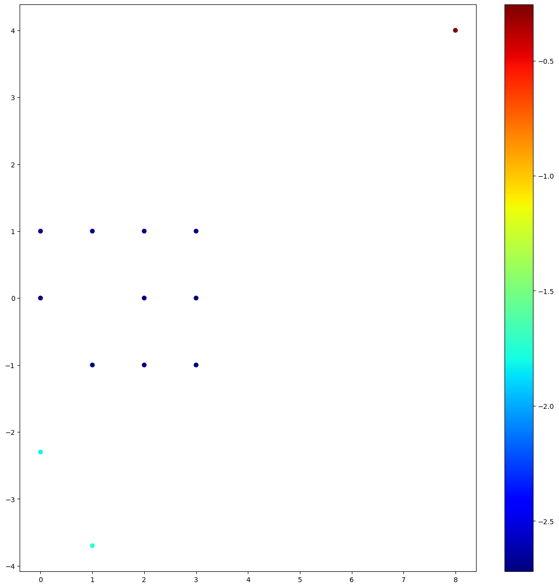
data_points = np.array([[0.0, 1.0], [1.0, 1.0], [2.0, 1.0], [3.0, 1.0],
                 [0.0, 0.0], [1.0, -3.70], [2.0, 0.0], [3.0, 0.0],
                 [0.0,-2.30], [1.0,-1.0], [2.0,-1.0], [3.0,-1.0],
                  [8.0, 4.0]
                ])
model = HVOF()
model.fit(data_points, mass_k = 2, KeepVolumeRatio = True)
scores = model.decision_scores_
print(scores)
model.visualize()

# Create a figure and axes
fig, ax = plt.subplots()
data = model.VolumeRatio
# Iterate over each row and create a boxplot
for i in range(data.shape[0]):
    row = data[i, :]
    mask = np.isnan(row)
    ax.boxplot(row[~mask], positions=[i + 1], vert=False, widths=0.5)
# Set labels and title
ax.set_xlabel("HVOF")
ax.set_ylabel("Data points")
ax.set_title("Boxplot of VolumeRatio distribution")
# Show the plot
plt.grid(True)
plt.show()
Output
[0.0658864  0.0658864  0.0658864  0.0658864  0.0658864  0.17635502
 0.0658864  0.0658864  0.16412078 0.06588641 0.06588641 0.06588641
 0.77389711]
Release history Release notifications | RSS feed


Download files
Download the file for your platform. If you're not sure which to choose, learn more about installing packages.
Source Distribution
Built Distribution
Filter files by name, interpreter, ABI, and platform.
If you're not sure about the file name format, learn more about wheel file names.
Copy a direct link to the current filters
File details
Details for the file pymof-0.7.0.tar.gz.
File metadata
- Download URL: pymof-0.7.0.tar.gz
- Upload date:
- Size: 17.2 kB
- Tags: Source
- Uploaded using Trusted Publishing? Yes
- Uploaded via: twine/6.1.0 CPython/3.13.7
File hashes
| Algorithm | Hash digest | |
|---|---|---|
| SHA256 |
723ad5441012ced318a23f3c537bb571a3a37a1f997587705c40dff27f6fc06b
|
|
| MD5 |
eb94a71304e0509f7b2a3e38f80d4a59
|
|
| BLAKE2b-256 |
de8e51cae84d7ed2a941ccbf408c05dfc06d9eb1322194e73303c4db377b2697
|
Provenance
The following attestation bundles were made for pymof-0.7.0.tar.gz:
Publisher:
workflows.yml on oakkao/pymof
-
Statement:
-
Statement type:
https://in-toto.io/Statement/v1 -
Predicate type:
https://docs.pypi.org/attestations/publish/v1 -
Subject name:
pymof-0.7.0.tar.gz -
Subject digest:
723ad5441012ced318a23f3c537bb571a3a37a1f997587705c40dff27f6fc06b - Sigstore transparency entry: 760833768
- Sigstore integration time:
-
Permalink:
oakkao/pymof@69f6860dc0e1bffa786ec40a03996986f16654a3 -
Branch / Tag:
refs/tags/v0.7.0 - Owner: https://github.com/oakkao
-
Access:
public
-
Token Issuer:
https://token.actions.githubusercontent.com -
Runner Environment:
github-hosted -
Publication workflow:
workflows.yml@69f6860dc0e1bffa786ec40a03996986f16654a3 -
Trigger Event:
release
-
Statement type:
File details
Details for the file pymof-0.7.0-py3-none-any.whl.
File metadata
- Download URL: pymof-0.7.0-py3-none-any.whl
- Upload date:
- Size: 15.1 kB
- Tags: Python 3
- Uploaded using Trusted Publishing? Yes
- Uploaded via: twine/6.1.0 CPython/3.13.7
File hashes
| Algorithm | Hash digest | |
|---|---|---|
| SHA256 |
df14052e64b464510e4a3b9979dde7891f011a1857a13c1527665998edaa8e4b
|
|
| MD5 |
8e5123179188ef03c20db650ba1c2c88
|
|
| BLAKE2b-256 |
4643f0436bae3084da4322c7b8698aad723eaa4570e60693c6535132fe3174b1
|
Provenance
The following attestation bundles were made for pymof-0.7.0-py3-none-any.whl:
Publisher:
workflows.yml on oakkao/pymof
-
Statement:
-
Statement type:
https://in-toto.io/Statement/v1 -
Predicate type:
https://docs.pypi.org/attestations/publish/v1 -
Subject name:
pymof-0.7.0-py3-none-any.whl -
Subject digest:
df14052e64b464510e4a3b9979dde7891f011a1857a13c1527665998edaa8e4b - Sigstore transparency entry: 760833772
- Sigstore integration time:
-
Permalink:
oakkao/pymof@69f6860dc0e1bffa786ec40a03996986f16654a3 -
Branch / Tag:
refs/tags/v0.7.0 - Owner: https://github.com/oakkao
-
Access:
public
-
Token Issuer:
https://token.actions.githubusercontent.com -
Runner Environment:
github-hosted -
Publication workflow:
workflows.yml@69f6860dc0e1bffa786ec40a03996986f16654a3 -
Trigger Event:
release
-
Statement type:






