A metallic waveguide mode solver

Project description
PyMWM


PyMWM is a metallic waveguide mode solver written in Python.
It provides the dispersion relation, i.e. the relation between propagation constant β = α + iγ (with phase constant α and attenuation constant γ) and angular frequency ω, for cylindrical waveguide and planer waveguide (slits). It also provides the distribution of mode fields. Codes for coaxial waveguides are under development.
Version
0.1.2
Install
Install and update using pip
$ pip install -U pymwm
Install using conda
$ conda install -c mnishida pymwm
Dependencies
- python 3
- numpy
- scipy
- pandas
- pytables
- ray
- matplotlib
- pyoptmat
Uninstall
$ pip uninstall pymwm
or
$ conda uninstall pymwm
Usage
Let's consider a cylindrical waveguide whose radius is 0.15μm filled with water (refractive index : 1.333) surrounded by gold. You can specify the materials by the parameters for PyOptMat. Wavelength range is set by the parameters 'wl_min' (which is set 0.5 μm here) and 'wl_max' (1.0 μm). PyMWM compute the dispersion relation the two complex values, ω (complex angular frequency) and β (propagation constant). The range of the imaginary part of ω is set from -2π/wl_imag to 0 with the parameter 'wl_imag'. Usually, the cylindrical waveguide mode is specified by two integers, n and m. The number of sets indexed by n and m are indicated by the parameters 'num_n' and 'num_m', respectively.
>>> import pymwm
>>> params = {
     'core': {'shape': 'cylinder', 'size': 0.15, 'fill': {'RI': 1.333}},
     'clad': {'model': 'gold_dl'},
     'bounds': {'wl_max': 1.0, 'wl_min': 0.5, 'wl_imag': 10.0},
     'modes': {'num_n': 6, 'num_m': 2}
     }
>>> wg = pymwm.create(params)
If the parameters are set for the first time, the creation of waveguide-mode object will take a quite long time, because a sampling survey of βs in the complex plane of ω will be conducted and the obtained data is registered in the database. The second and subsequent creations are done instantly. You can check the obtained waveguide modes in the specified range by showing the attribute 'modes';
>>> wg.modes
{'h': [('E', 1, 1),
  ('E', 2, 1),
  ('E', 3, 1),
  ('E', 4, 1),
  ('M', 0, 1),
  ('M', 1, 1)],
 'v': [('E', 0, 1),
  ('E', 1, 1),
  ('E', 2, 1),
  ('E', 3, 1),
  ('E', 4, 1),
  ('M', 1, 1)]}
where 'h' ('v') means that the modes have horizontally (vertically) oriented electric fields on the x axis. The tuple (pol, n, m) with pol being 'E' or 'M' indicates TE-like or TM-like mode indexed by n and m. You can get β at ω=8.0 rad/μm for TM-like mode with n=0 and m=1 by
>>> wg.beta(8.0, ('M', 0, 1))
(0.06187318716518497+10.363105296313996j)
and for TE-like mode with n=1 and m=2 by
>>> wg.beta(8.0, ('E', 1, 2))
(0.14261514314942403+19.094726281995463j)
For more information, see the examples notebook.
Examples
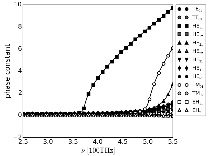
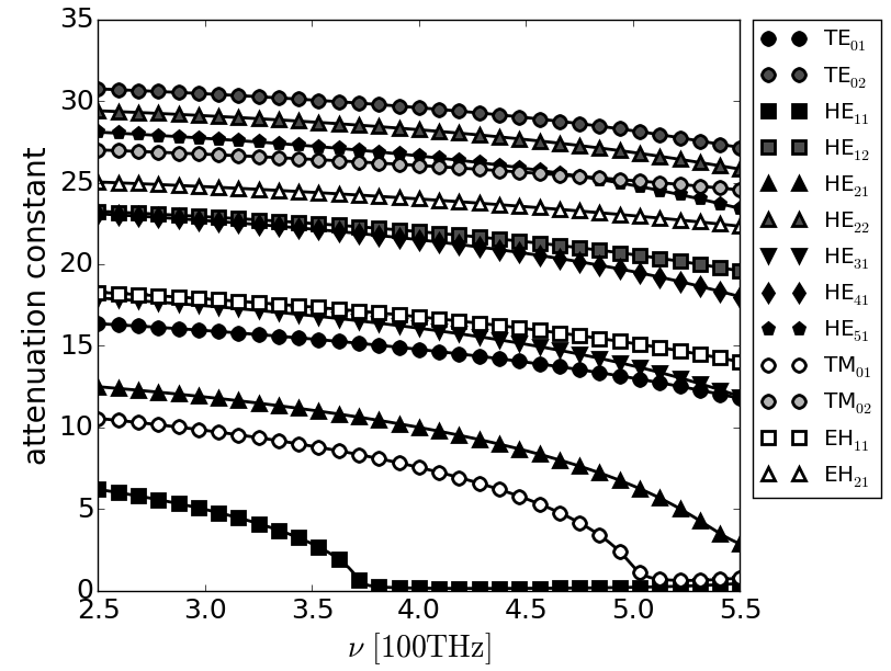
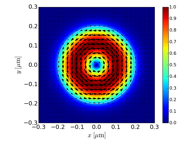
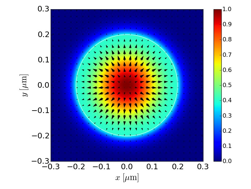
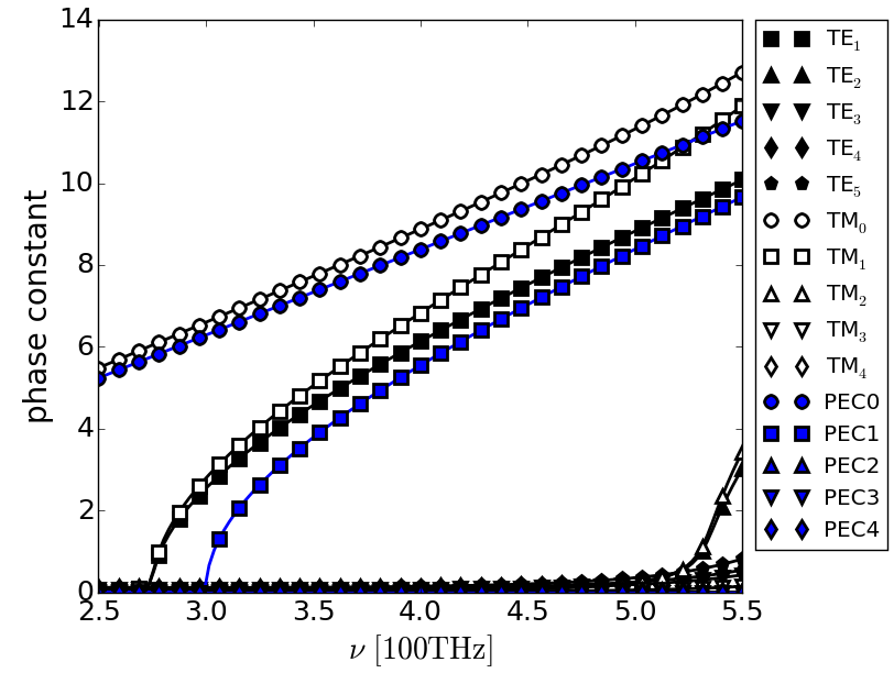
Cylindrical waveguide
Propagation constants
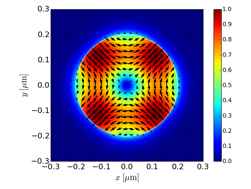
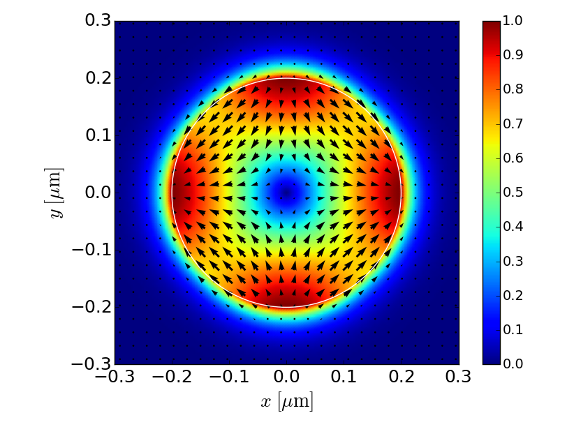
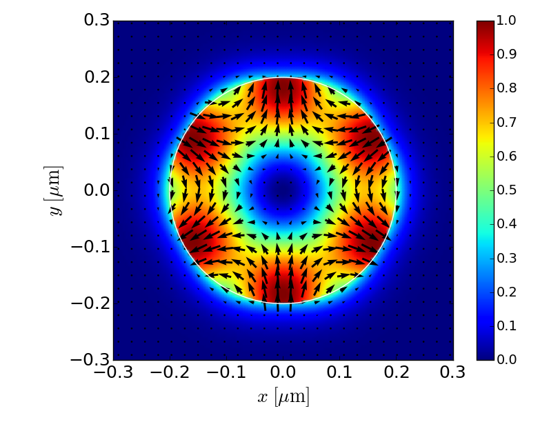
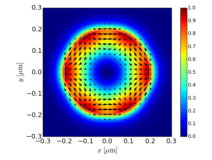
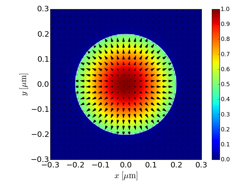
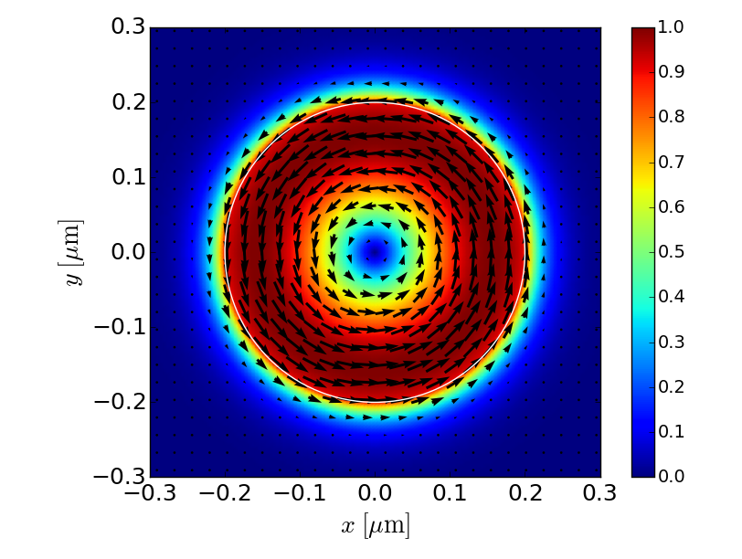
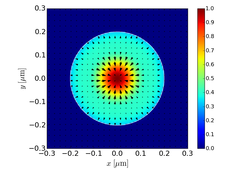
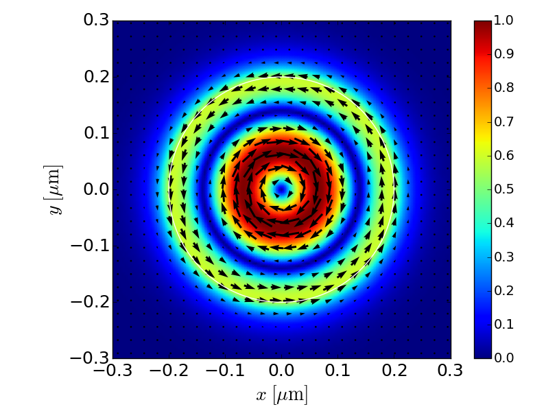
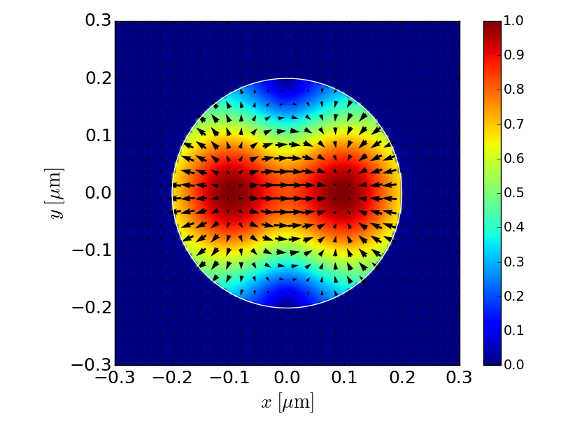
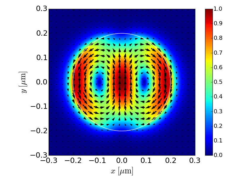
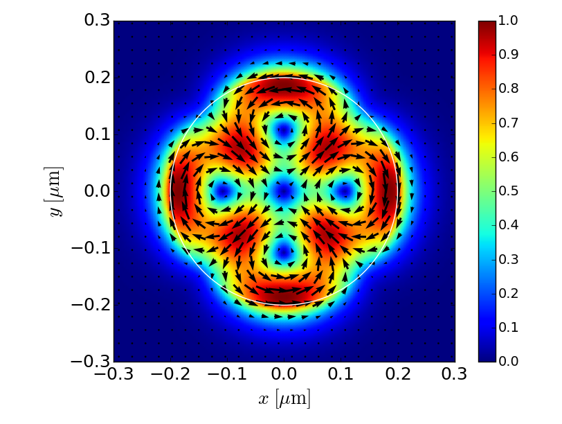
Electric field and magnetic field distributions
- TE01
- HE11
- HE12
- HE21
- HE31
- TM01
- TM02
- EH11
- EH21
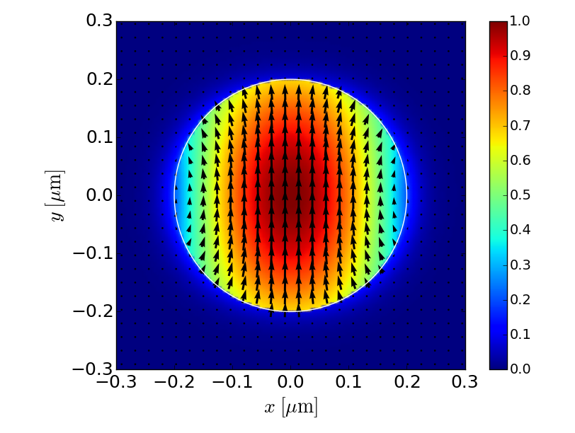
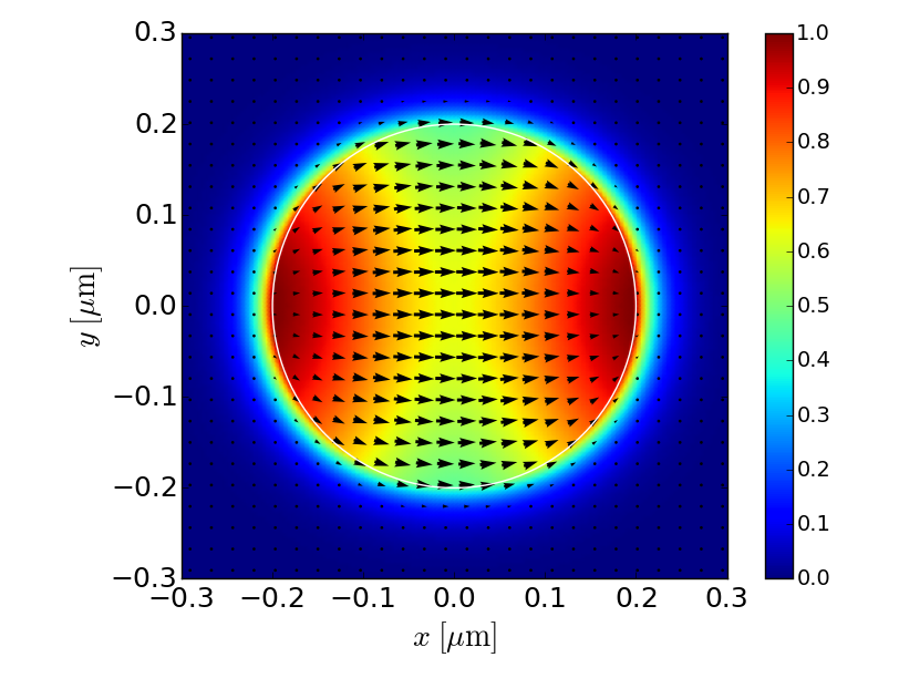
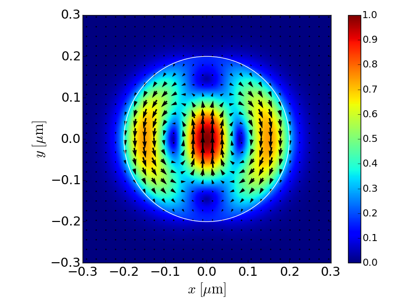
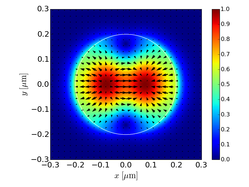

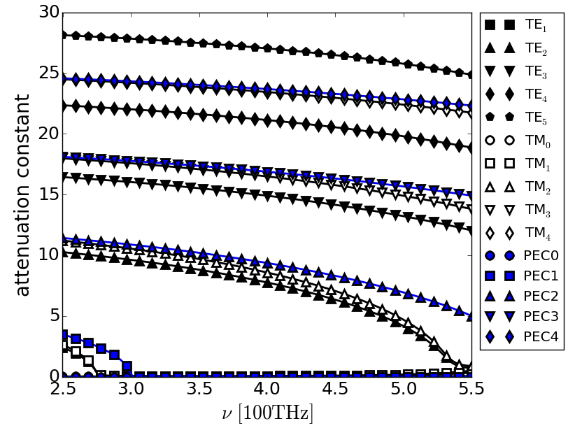
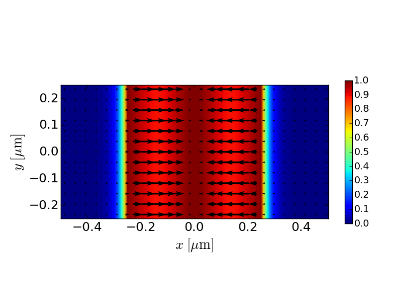
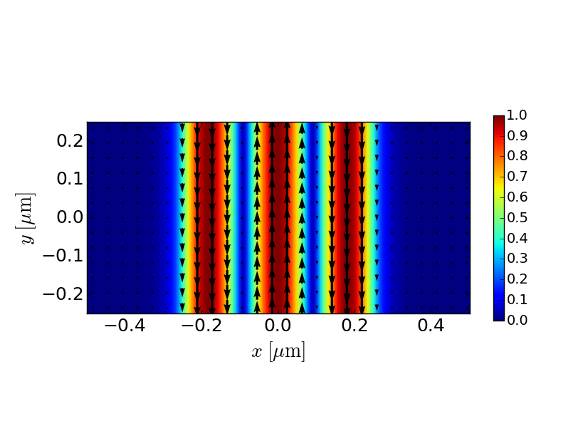
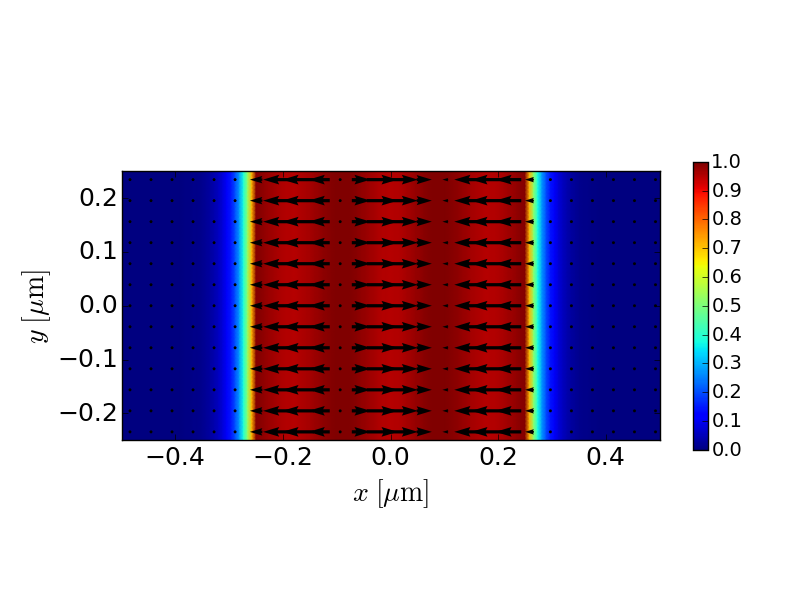
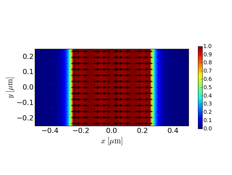
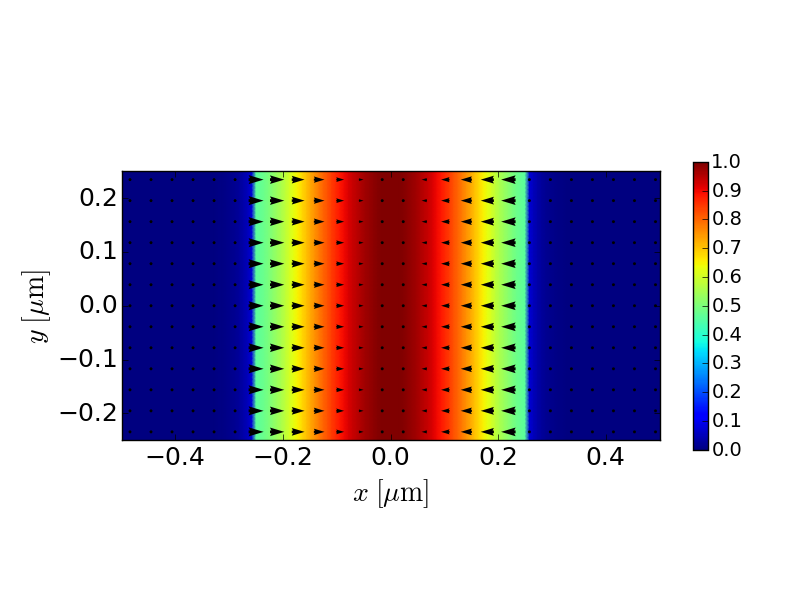
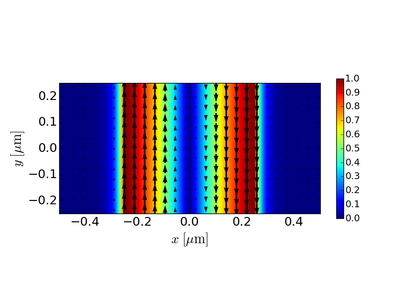
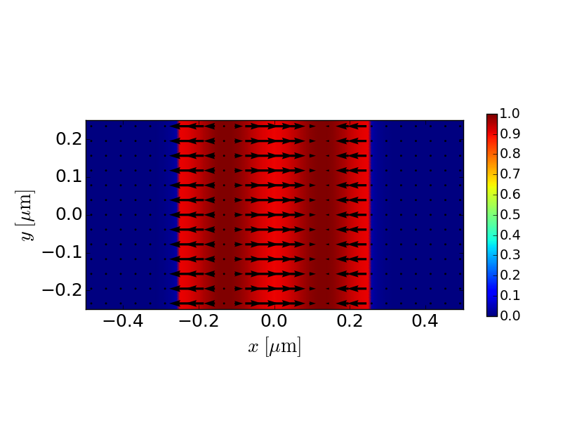
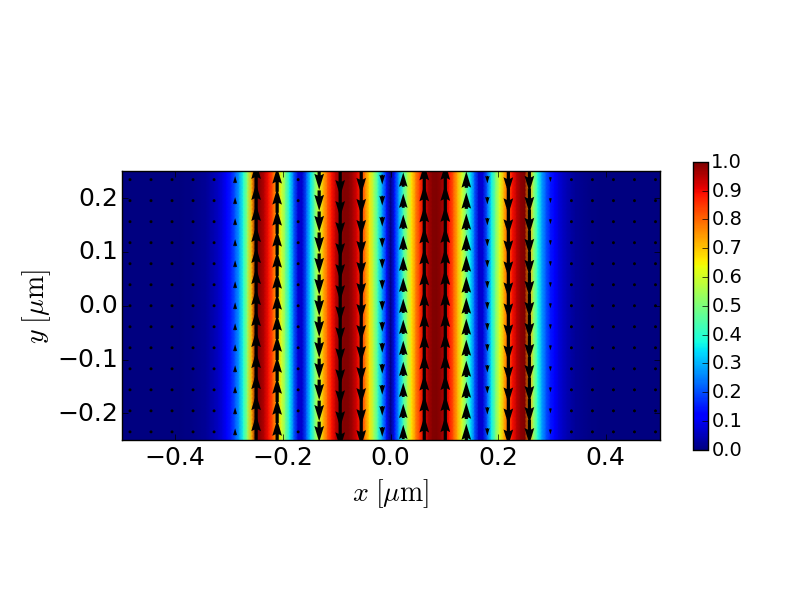
Slit waveguide
Propagation constants
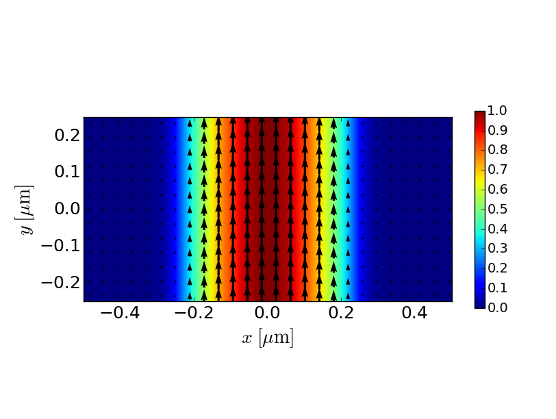
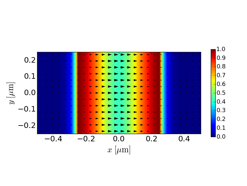
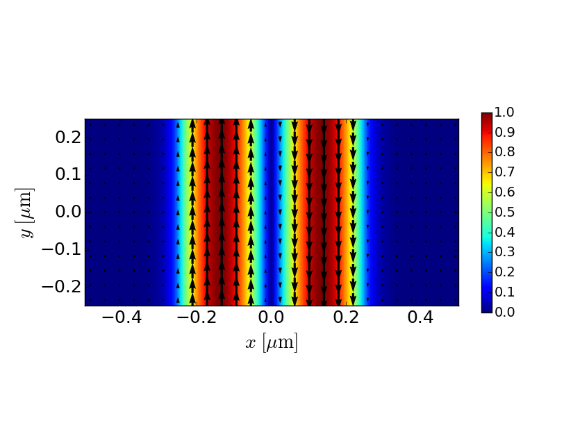
Electric field and magnetic field distributions
- TE1
- TE2
- TE3
- TE4
- TM0
- TM1
- TM2
- TM3


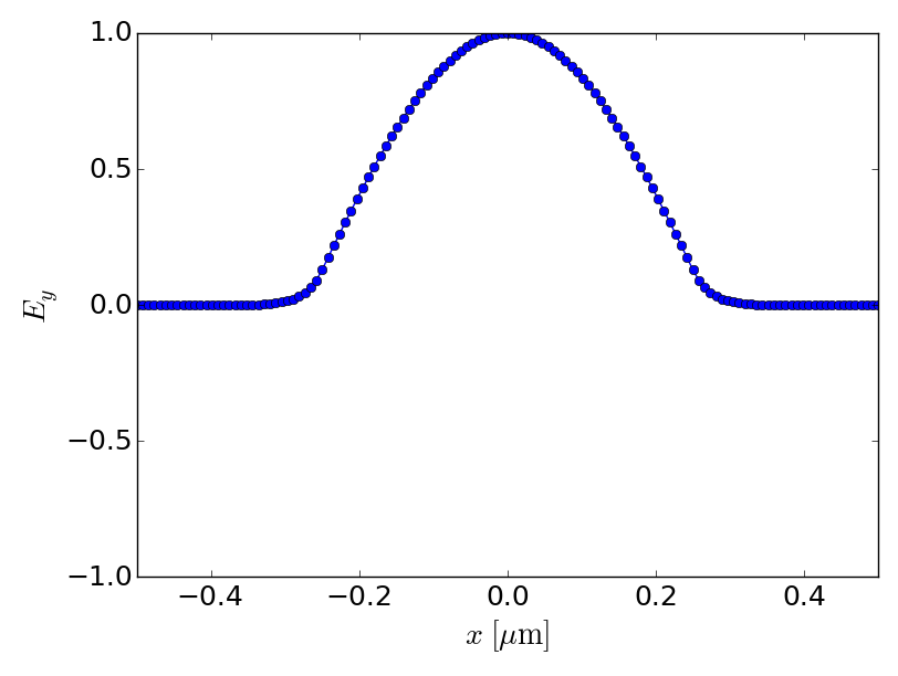
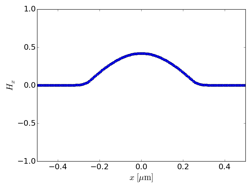
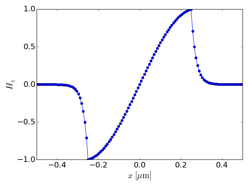
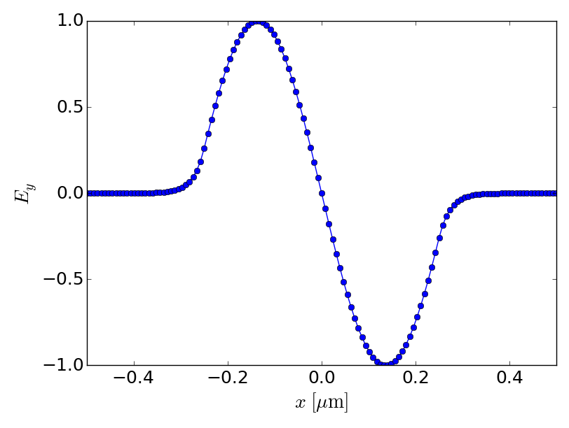
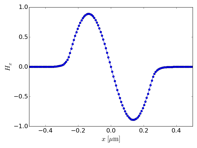
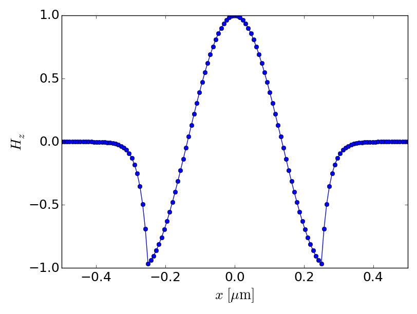
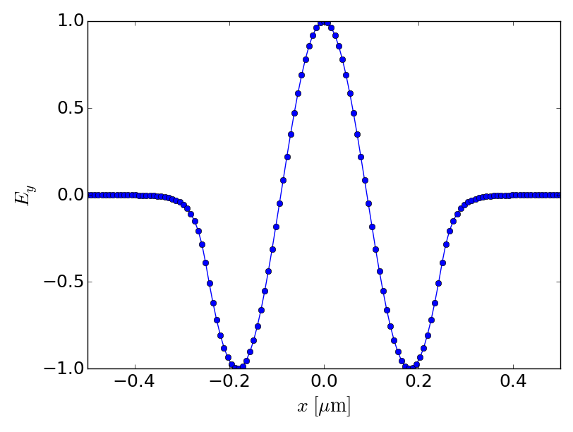
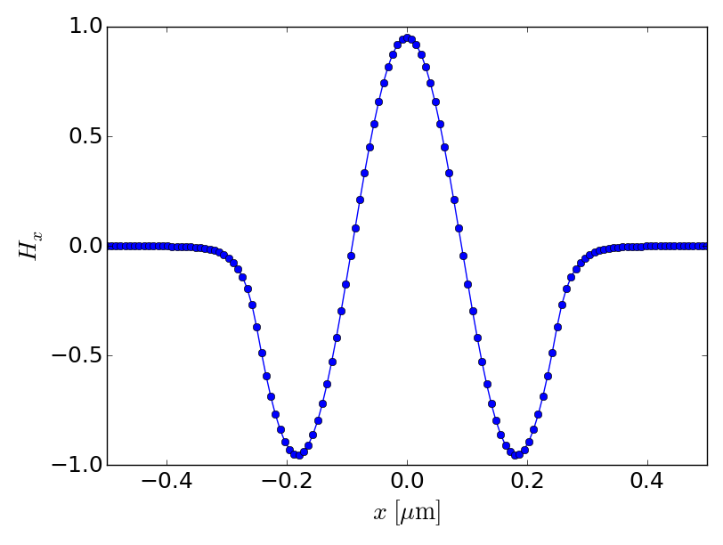
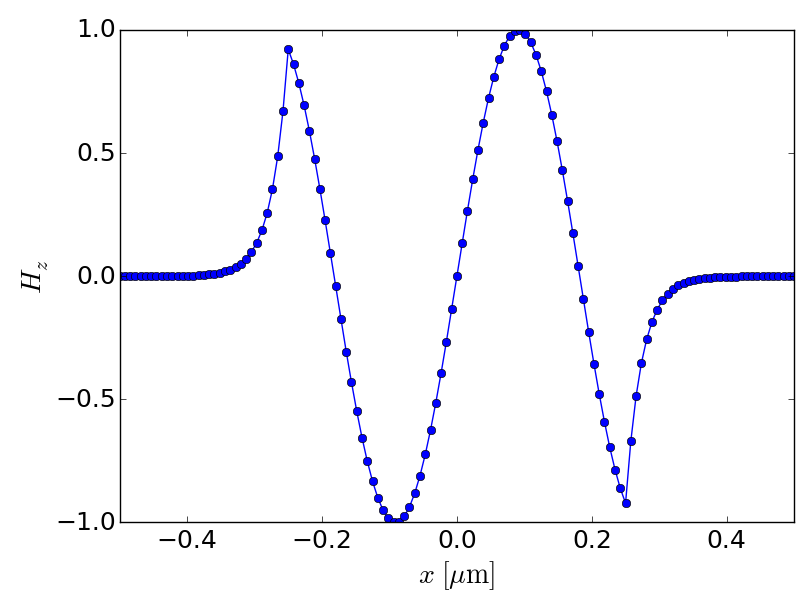
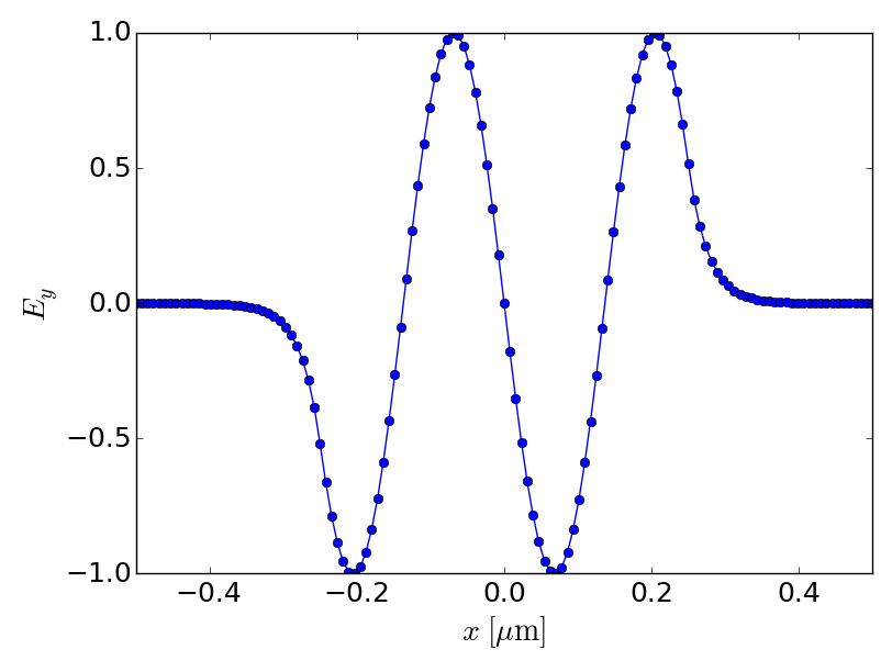
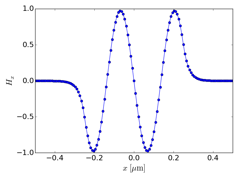
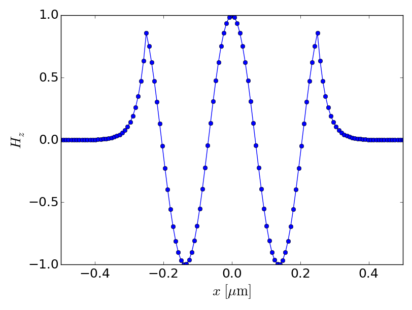
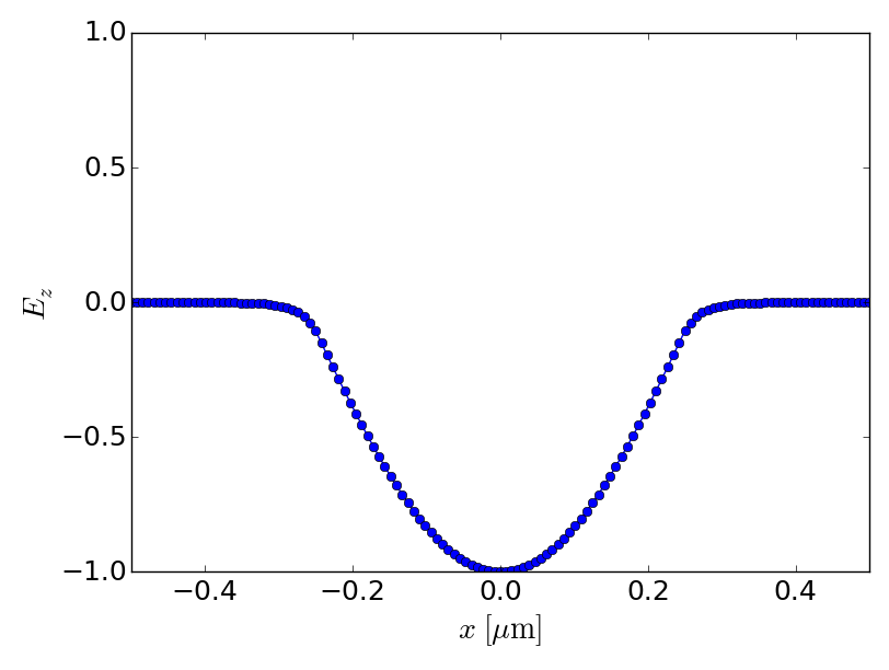
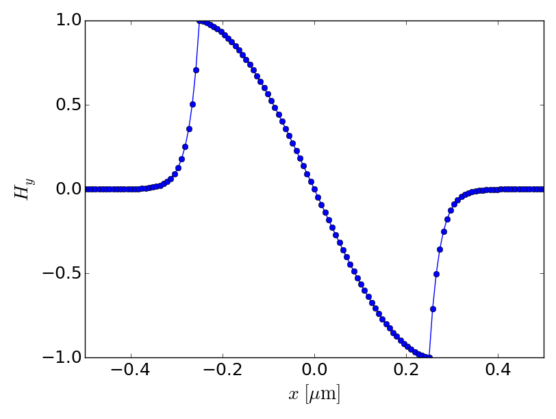
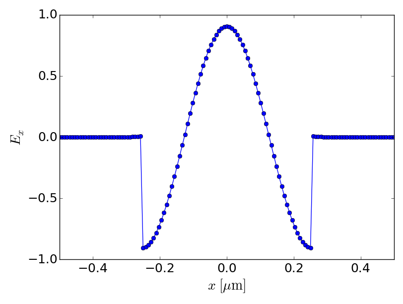
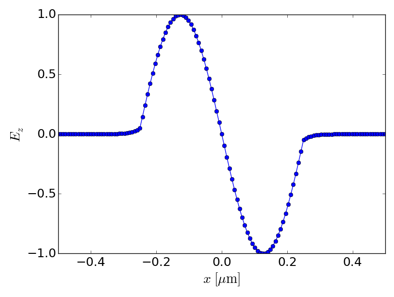
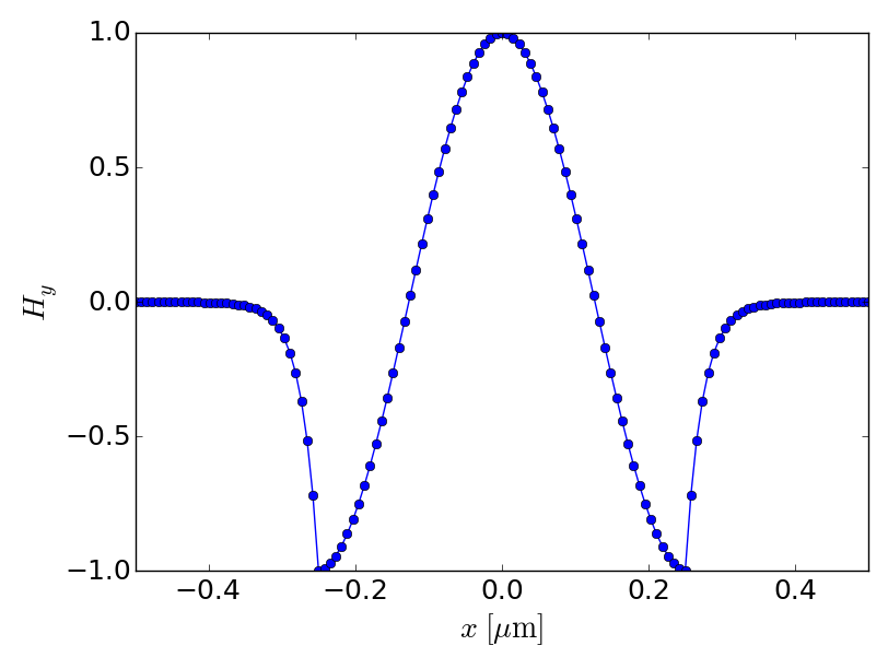
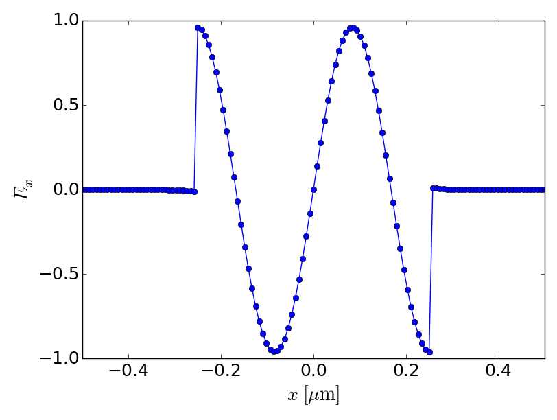
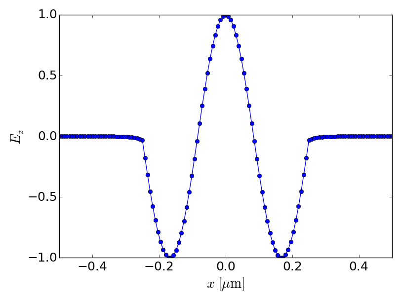
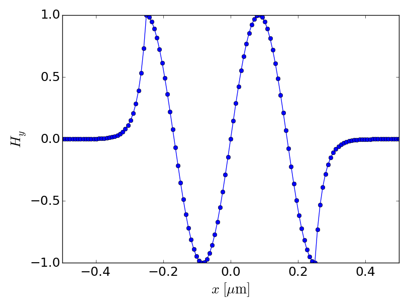
Ey, Hx and Hz distributions on x axis
- TE1
- TE2
- TE3
- TE4
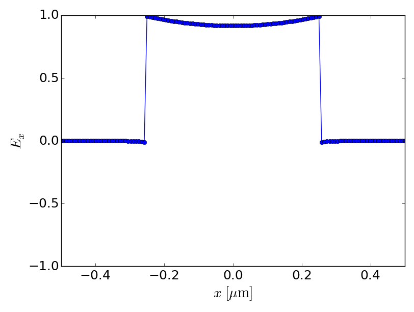
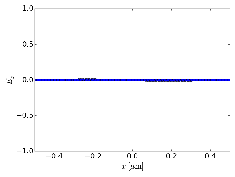
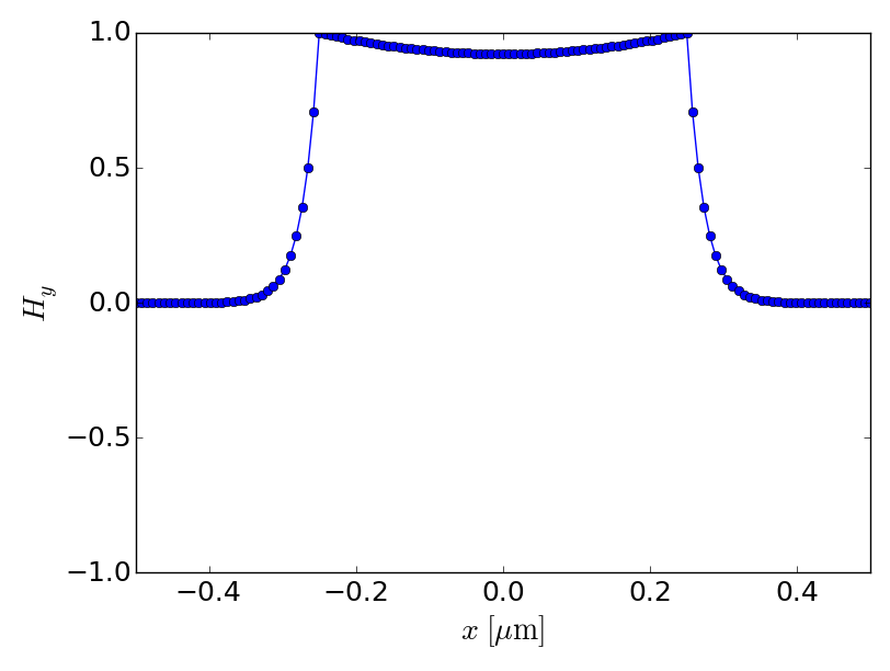
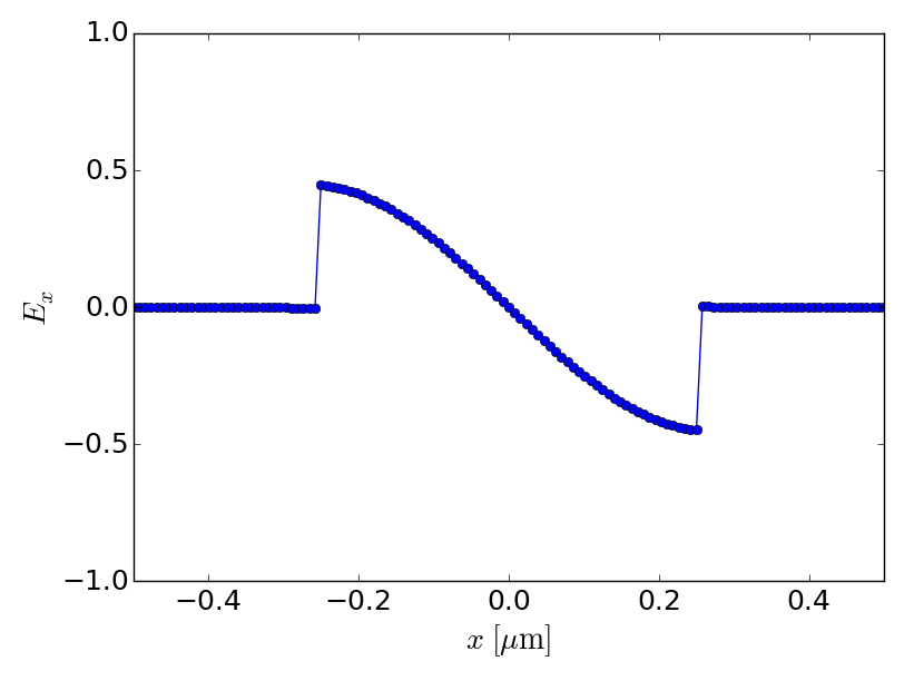
Ex, Ez and Hy distributions on x axis
- TM0
- TM1
- TM2
- TM3
Release history Release notifications | RSS feed


Download files
Download the file for your platform. If you're not sure which to choose, learn more about installing packages.
Source Distribution
File details
Details for the file pymwm-0.1.2.tar.gz.
File metadata
- Download URL: pymwm-0.1.2.tar.gz
- Upload date:
- Size: 6.0 MB
- Tags: Source
- Uploaded using Trusted Publishing? No
- Uploaded via: twine/3.4.2 importlib_metadata/4.6.4 pkginfo/1.7.1 requests/2.26.0 requests-toolbelt/0.9.1 tqdm/4.62.1 CPython/3.9.6
File hashes
| Algorithm | Hash digest | |
|---|---|---|
| SHA256 |
7a145fde6e79e32b1e27be76d26495319215d59601b3a5d37e047ef0c5874cc6
|
|
| MD5 |
26b51f79bb0efed895cfeb6d3a9c0bb7
|
|
| BLAKE2b-256 |
919fd83c38422f360a2000793017b63f34a86eeb142f90443b9716ca2e24e50e
|


