A python implementation of the Principal Component Geostatistical Approach (PCGA) for large scale inversion.

Project description
pyPCGA


🐍 A python implementation of the Principal Component Geostatistical Approach (PCGA) for large scale inversion.
The complete and up to date documentation can be found here: https://pypcga.readthedocs.io.
📖 Courses and theory
Please check out the UH CEE696 course on data assimilation
As well as the theory description.
⚙️ Implemented features:
Direct inversion with Cholesky (practical up to 100 obs. TODO).
Exact preconditioner construction (inverse of cokriging/saddle-point matrix) using generalized eigendecomposition [Lee et al., WRR 2016, Saibaba et al, NLAA 2016]
Fast hyperparameter tuning and predictive model validation using cR/Q2 criteria [Kitanidis, Math Geol 1991]
Fast posterior variance/std computation using exact preconditioner
💻 Example Notebooks
1D linear inversion example below will be helpful to understand how pyPCGA can be implemented. Please check Google Colab examples.
1D linear inversion example (from Stanford 362G course) Google Colab example 1
1D nonlinear inversion example (from Stanford 362G course) Google Colab example 2
Hydraulic conductivity estimation example using USGS-FloPy (MODFLOW) [Lee and Kitanidis, 2014] Google Colab example 3
Tracer tomography example using Crunch (with Mahta Ansari from UIUC Druhan Lab)
Bathymetry estimation example using STWAVE (with USACE-ERDC-CHL)
Permeability estimation example using TOUGH2 (with Amalia Kokkianki, USFCA)
Electrical conductivity estimation example using magnetotelluric (MT) survey with MARE2DEM (with Niels Grobbe, UHM)
DNAPL plume estimation using hydraulic head, self-potential (SP) and partitioning tracer data (with Xueyuan Kang et al.)
ERT example using E4D will be completed soon.
🚀 Quick start with a 2D toy example
To install pypcga, the easiest way is through pip:
pip install pypcga[examples]Or alternatively using conda
conda install pypcga[examples]You might also clone the repository and install from source
pip install -e .[examples]To illustrate pypcga and expose its main features, let’s use a toy 2D example. The forward is simple static smoohting (non linear but with no time dependance) and is used both to produce a reference field from which observations will be sampled and the inversion.
Import the required modules
import matplotlib.pyplot as plt
import numpy as np
import scipy as sp
import covmats
import pypcga
from pypcga._utils import NDArrayFloat
import logging
import nested_grid_plotter as ngp
Apply nice parameters for the plots
ngp.apply_nice_default_rc_params()Create some logging.Logger instances to illustrate how to use them in a complex workflow
# Create loggers
main_logger = logging.getLogger("main")
main_logger.setLevel(logging.INFO)
pcga_logger = logging.getLogger("PCGA")
pcga_logger.setLevel(logging.INFO)
main_logger.info("This is the main logger")
pcga_logger.info("This is the PCGA logger")
Let’s use an example provided by covmats. Here, the prior covariance matrix, \(\mathbf{C}_{\mathrm{prior}}\) is represented as a sparse factorization of its inverse \(\mathbf{C}_{\mathrm{prior}}^{-1}\) with \(\mathbf{LDL}^{\mathrm{T}} = \mathbf{PC}_{\mathrm{prior}}^{-1}\mathbf{P}^{\mathrm{T}}\). This is wrapped in the :py:class:`**covmats.CovViaSparsePrecisionCholesky instance we create:
cov_prior = covmats.CovViaSparsePrecisionCholesky(
covmats.load_precision_example_4225x_SCF()
)
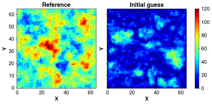
cov_prior<4225x4225 CovViaSparsePrecisionCholesky with dtype=float64>The covariance matrix has shape (4225, 4225) , let’s define a square domain (65, 65) and perform a non conditional simulation using our prior. We set a mean @ 50 and display it:
# Domain dimensions
nx = ny = int(np.sqrt(cov_prior.shape[0]))

# Non conditonal simulation -> change the random states (seeds) to obtain different fields
simu_ = cov_prior.sample_mvnormal(shape=(1,), random_state=2026).reshape(ny, nx).T
mean= 50.0
# Reference field
s_ref = np.abs(simu_ + mean)
# Initial guess
s_init = np.abs(cov_prior.sample_mvnormal(shape=(1,), random_state=15653).reshape(ny, nx).T)

plotter = ngp.Plotter(fig=plt.figure(figsize=(9, 4.3)),builder=ngp.SubplotsMosaicBuilder([["ax11", "ax12"]], sharex=True, sharey=True))
ngp.multi_imshow(
    plotter.axes,
    plotter.fig,
    data={"Reference": s_ref, "Initial guess": s_init},
    xlabel="X", ylabel="Y", imshow_kwargs=dict(cmap=plt.get_cmap("jet"),
    aspect="equal",
    vmin=0.0,
    vmax=120,)
)
The forward is simple static smoohting (non linear but with no time dependance) and is used both to produce a reference field from which observations will be sampled and the inversion. Here, forward_multiple is just the generalization to an ensemble of vectors, i.e., in PCGA, most forward calls for an iteration can be performed in parallel. But it is the responsibility of the user to decide and implement the sequential forward computation (a simple for loop as here) or the parallelized computation (with mpi, multiprocessing, joblib or whatever tool that suits best).
# Data transform operator
def transform_model(x: NDArrayFloat) -> NDArrayFloat:
    """Transform the input space into the output space."""
    return sp.ndimage.gaussian_filter(4.0 * x**2, sigma=2.0)

# Sampling operator
def sample_d(d: NDArrayFloat, sampling_fraction: float = 0.05) -> NDArrayFloat:
    """
    Sample within a vector.

    Parameters
    ----------
    d : NDArrayFloat
        Values to sample.
    sampling_fraction : float, optional
        Fraction of the values to sample, by default 0.05.
    """
    return d.ravel("F")[:: int(d.size / (sampling_fraction * 1000))]

def forward(x: NDArrayFloat) -> NDArrayFloat:
    """
    Forward model (data transform + sampling in the output space).

    Parameters
    ----------
    x : NDArrayFloat
        Input parameters vector with size (N_s).

    Returns
    -------
    NDArrayFloat
    """
    return sample_d(transform_model(x))

def forward_multiple(X: NDArrayFloat, *args, **kargs) -> NDArrayFloat:
    """
    Return the results of the forward for an ensemble of input vectors.

    Parameters
    ----------
    X : _type_
        Input vectors as a matrix with size (N_s, N_e), N_s being the number of
        parameter values per vector and N_e the number of vectors, aka the ensemble
        size.

    Returns
    -------
    NDArrayFloat
        _description_
    """
    res = []
    _X = np.atleast_2d(X.T)
    for i in range(_X.shape[0]):
        res.append(forward(_X[i, :].reshape(nx, ny, order="F")))
    return np.vstack(res).T

# The input vector much match a flatten version of the field (Here, 2D -> 1D).
obs = forward_multiple(s_ref.ravel())[:, 0]
# Some test to check that all works as expected
s_ens = np.vstack([s_ref.ravel("F"), s_init.ravel("F")]).T
assert s_ens.shape == (nx * ny, 2)
d_pred = forward_multiple(s_ens)
assert d_pred.shape == (obs.size, 2)
np.testing.assert_almost_equal(d_pred[:, 0], obs)
Define the covariance matrix of observation errors (cov_obs). To illustrate a complex case, the matrix is assumed non diagonal.
n = np.size(obs)
amplitude = (np.max(obs) - np.min(obs))

# CASE 1: diagonal covariance matrix (this is the simplest case)
# 10% error on the observations
# cov_obs = covmats.CovViaDiagonal(
#     np.ones(n) * amplitude ** 2
# )

# CASE 2: non diagonal through Cholesky
L = np.zeros((n ,n), dtype=np.float64)
# Add some random non-zero covariances
for i in range(n):
    for j in range(i + 1, n):
        if np.random.rand() < 0.1:  # 10% chance of non-zero covariance
            cov = np.random.uniform(-0.05, 0.05) * amplitude
            L[i, j] = cov
            L[j, i] = cov  # symmetry
# Add non zero diagonal
L.flat[:: n + 1] = amplitude * 0.1
# Make it lower triangular and define the covariance as a cholesky factorization
cov_obs = covmats.CovViaCholesky(np.tril(L))

# Show the dense matrix
plt.imshow(cov_obs.todense())
plt.colorbar()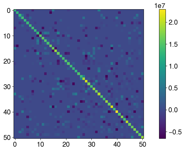
Perturb the observations to avoid the inverse crime (using the same forward to generate the synthetic data and perform the inversion makes the problem well posed and simple to solve. Adding noise mitigates it a bit).
obs_perturb = (
    obs + cov_obs.sample_mvnormal([1], random_state=np.random.default_rng(2151))[0]
)
# Plot the non perturbed observations vs perturbed ones
# The perturbed ones will be used for the inversion
pl = ngp.Plotter()
lims = (np.min(obs), np.max(obs))
diff = lims[1] - lims[0]
lims = (lims[0]- 0.2 * diff, lims[1]+ 0.2 * diff)
pl.axes[0].plot(lims, lims, color="r")
pl.axes[0].scatter(obs_perturb, obs)
pl.axes[0].set_xlabel("Perturbed values (observations)")
pl.axes[0].set_ylabel("Values")
pl.axes[0].set_aspect("equal")
pl.axes[0].set_xlim(lims)
pl.axes[0].set_ylim(lims)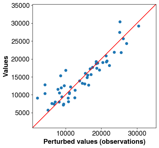
The next step is to factorize the parameters covariance matrix. The number of principal component is set to 50.
eig_mat = covmats.eigen_factorize_cov_mat(cov_prior, n_pc=50)
assert eig_mat.n_pts == 4225
It is then possible to check the explained variance retained as a function of the number of principal components kept and adjust the number accordingly. The Eigen factorization is a compression of the information. The less principal components kept, the less foward calls needed in PCGA which is critical when dealing with expensive forward models (e.g., when relying on high fidelity reervoir simlations) but the more “smoohting” it introduces (we can see this as loss of details in the inversion).
plt.plot(np.cumsum(covmats.get_explained_var(eig_mat.eig_vals, cov_prior)) * 100.0)
plt.xlabel("Number of principal components (PC)")
plt.ylabel("Cumulative explained variance(%)")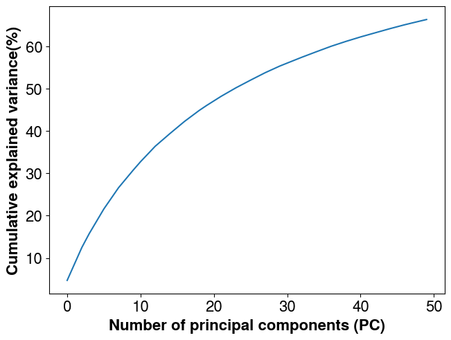
Create the PCGA instance
solver = pypcga.PCGA(
    s_init=s_init.ravel("F"),
    obs=obs_perturb,
    cov_obs=cov_obs,
    forward_model=forward_multiple,
    Q=eig_mat,
    maxiter=5,
    is_lm=True,
    is_direct_solve=False,
    prior_s_var=None,
    random_state=2026,
    logger=pcga_logger,
)
# Sanity checks just for the tests
assert solver.s_dim == nx * ny
assert solver.d_dim == obs.size
INFO:PCGA:##### PCGA Inversion #####
INFO:PCGA:##### 1. Initialize forward and inversion parameters
INFO:PCGA:------------ Inversion Parameters -------------------------
INFO:PCGA: Number of unknowns : 4225
INFO:PCGA: Number of observations : 51
INFO:PCGA: Number of principal components (n_pc) : 50
INFO:PCGA: Maximum Gauss-Newton iterations : 5
INFO:PCGA: Machine eps (delta = sqrt(eps)) : 1e-08
INFO:PCGA: Minimum model change (restol) : 0.01
INFO:PCGA: Minimum obj fun change (ftol) : 0.0
INFO:PCGA: Target obj fun (ftarget) : None
INFO:PCGA: Levenberg-Marquardt (is_lm) : True
INFO:PCGA: Minimum LM solution (lm_smin) : None
INFO:PCGA: Maximum LM solution (lm_smax) : None
INFO:PCGA: Maximum LM iterations (max_it_lm) : 16
INFO:PCGA: Line search : False
INFO:PCGA:-----------------------------------------------------------Run the inversion process
s_hat, simul_obs, post_diagv, iter_best = solver.run()INFO:PCGA:##### 2. Start PCGA Inversion #####
INFO:PCGA:-- evaluate initial solution
INFO:PCGA:** LS objfun 0.5 (obs. diff.)^T R^{-1}(obs. diff.) : 1.149e+03
INFO:PCGA:** norm LS objfun 0.5 / nobs (obs. diff.)^T R^{-1}(obs. diff.) : 2.253e+01
INFO:PCGA:** RMSE (norm(obs. diff.)/sqrt(nobs)) : 1.480e+04
INFO:PCGA:** norm RMSE (norm(obs. diff./sqrtR)/sqrt(nobs)) : 6.713e+00
INFO:PCGA:** objective function (no beta) : 1.163e+03
INFO:PCGA:
INFO:PCGA:***** Iteration 1 ******
INFO:PCGA:computed Jacobian-Matrix products in : 2.598e-02 s
INFO:PCGA:Use Krylov subspace iterative solver for saddle-point (cokrigging) system
INFO:PCGA:Preconditioner construction using Generalized Eigen-decomposition
INFO:PCGA:Time for data covarance construction :3.53e-02 sec
INFO:PCGA:Evaluate the 5 LM solutions
INFO:PCGA:5 objective value evaluations
INFO:PCGA:solution obj=4.00e+03 (cov_obs inflation factor=1.00e+03)
INFO:PCGA:- Geostat. inversion at iteration 1 is 1 sec
INFO:PCGA:** LS objfun 0.5 (obs. diff.)^T R^{-1}(obs. diff.) : 3.998e+03
INFO:PCGA:** norm LS objfun 0.5 / nobs (obs. diff.)^T R^{-1}(obs. diff.) : 7.840e+01
INFO:PCGA:** RMSE (norm(obs. diff.)/sqrt(nobs)) : 2.578e+04
INFO:PCGA:** norm RMSE (norm(obs. diff./sqrtR)/sqrt(nobs)) : 1.252e+01
INFO:PCGA:** objective function : 3.998e+03
INFO:PCGA:** relative L2-norm diff btw sol 0 and sol 1 : 3.718e+00
INFO:PCGA:start posterior variance computation
INFO:PCGA:Preconditioner construction using Generalized Eigen-decomposition
INFO:PCGA:Time for data covarance construction :5.30e-02 sec
INFO:PCGA:posterior diag. computed in 2.503e-01 s
INFO:PCGA:
INFO:PCGA:***** Iteration 2 ******
INFO:PCGA:computed Jacobian-Matrix products in : 1.050e-02 s
INFO:PCGA:Use Krylov subspace iterative solver for saddle-point (cokrigging) system
INFO:PCGA:Preconditioner construction using Generalized Eigen-decomposition
INFO:PCGA:Time for data covarance construction :1.60e-02 sec
INFO:PCGA:Evaluate the 5 LM solutions
INFO:PCGA:5 objective value evaluations
INFO:PCGA:solution obj=1.48e+02 (cov_obs inflation factor=1.00e+00)
INFO:PCGA:- Geostat. inversion at iteration 2 is 0 sec
INFO:PCGA:== iteration 2 summary ==
INFO:PCGA:** LS objfun 0.5 (obs. diff.)^T R^{-1}(obs. diff.) : 1.369e+02
INFO:PCGA:** norm LS objfun 0.5 / nobs (obs. diff.)^T R^{-1}(obs. diff.) : 2.684e+00
INFO:PCGA:** RMSE (norm(obs. diff.)/sqrt(nobs)) : 4.868e+03
INFO:PCGA:** norm RMSE (norm(obs. diff./sqrtR)/sqrt(nobs)) : 2.317e+00
INFO:PCGA:** objective function : 1.481e+02
INFO:PCGA:** relative L2-norm diff btw sol 1 and sol 2 : 3.233e-01
INFO:PCGA:start posterior variance computation
INFO:PCGA:Preconditioner construction using Generalized Eigen-decomposition
INFO:PCGA:Time for data covarance construction :5.52e-02 sec
INFO:PCGA:posterior diag. computed in 2.798e-01 s
INFO:PCGA:
INFO:PCGA:***** Iteration 3 ******
INFO:PCGA:computed Jacobian-Matrix products in : 3.163e-02 s
INFO:PCGA:Use Krylov subspace iterative solver for saddle-point (cokrigging) system
INFO:PCGA:Preconditioner construction using Generalized Eigen-decomposition
INFO:PCGA:Time for data covarance construction :2.98e-02 sec
INFO:PCGA:Evaluate the 5 LM solutions
INFO:PCGA:5 objective value evaluations
INFO:PCGA:solution obj=2.86e+01 (cov_obs inflation factor=1.00e+00)
INFO:PCGA:- Geostat. inversion at iteration 3 is 0 sec
INFO:PCGA:== iteration 3 summary ==
INFO:PCGA:** LS objfun 0.5 (obs. diff.)^T R^{-1}(obs. diff.) : 8.550e+00
INFO:PCGA:** norm LS objfun 0.5 / nobs (obs. diff.)^T R^{-1}(obs. diff.) : 1.676e-01
INFO:PCGA:** RMSE (norm(obs. diff.)/sqrt(nobs)) : 1.706e+03
INFO:PCGA:** norm RMSE (norm(obs. diff./sqrtR)/sqrt(nobs)) : 5.790e-01
INFO:PCGA:** objective function : 2.857e+01
INFO:PCGA:** relative L2-norm diff btw sol 2 and sol 3 : 1.256e-01
INFO:PCGA:start posterior variance computation
INFO:PCGA:Preconditioner construction using Generalized Eigen-decomposition
INFO:PCGA:Time for data covarance construction :7.53e-02 sec
INFO:PCGA:posterior diag. computed in 2.893e-01 s
INFO:PCGA:
INFO:PCGA:***** Iteration 4 ******
INFO:PCGA:computed Jacobian-Matrix products in : 3.353e-02 s
INFO:PCGA:Use Krylov subspace iterative solver for saddle-point (cokrigging) system
INFO:PCGA:Preconditioner construction using Generalized Eigen-decomposition
INFO:PCGA:Time for data covarance construction :2.89e-02 sec
INFO:PCGA:Evaluate the 5 LM solutions
INFO:PCGA:5 objective value evaluations
INFO:PCGA:solution obj=2.79e+01 (cov_obs inflation factor=1.00e+00)
INFO:PCGA:- Geostat. inversion at iteration 4 is 0 sec
INFO:PCGA:== iteration 4 summary ==
INFO:PCGA:** LS objfun 0.5 (obs. diff.)^T R^{-1}(obs. diff.) : 7.601e+00
INFO:PCGA:** norm LS objfun 0.5 / nobs (obs. diff.)^T R^{-1}(obs. diff.) : 1.490e-01
INFO:PCGA:** RMSE (norm(obs. diff.)/sqrt(nobs)) : 1.696e+03
INFO:PCGA:** norm RMSE (norm(obs. diff./sqrtR)/sqrt(nobs)) : 5.460e-01
INFO:PCGA:** objective function : 2.790e+01
INFO:PCGA:** relative L2-norm diff btw sol 3 and sol 4 : 1.197e-02
INFO:PCGA:start posterior variance computation
INFO:PCGA:Preconditioner construction using Generalized Eigen-decomposition
INFO:PCGA:Time for data covarance construction :7.28e-02 sec
INFO:PCGA:posterior diag. computed in 2.728e-01 s
INFO:PCGA:
INFO:PCGA:***** Iteration 5 ******
INFO:PCGA:computed Jacobian-Matrix products in : 1.885e-02 s
INFO:PCGA:Use Krylov subspace iterative solver for saddle-point (cokrigging) system
INFO:PCGA:Preconditioner construction using Generalized Eigen-decomposition
INFO:PCGA:Time for data covarance construction :2.59e-02 sec
INFO:PCGA:Evaluate the 5 LM solutions
INFO:PCGA:5 objective value evaluations
INFO:PCGA:solution obj=2.79e+01 (cov_obs inflation factor=1.00e+00)
INFO:PCGA:- Geostat. inversion at iteration 5 is 0 sec
INFO:PCGA:== iteration 5 summary ==
INFO:PCGA:** LS objfun 0.5 (obs. diff.)^T R^{-1}(obs. diff.) : 7.647e+00
INFO:PCGA:** norm LS objfun 0.5 / nobs (obs. diff.)^T R^{-1}(obs. diff.) : 1.499e-01
INFO:PCGA:** RMSE (norm(obs. diff.)/sqrt(nobs)) : 1.701e+03
INFO:PCGA:** norm RMSE (norm(obs. diff./sqrtR)/sqrt(nobs)) : 5.476e-01
INFO:PCGA:** objective function : 2.790e+01
INFO:PCGA:** relative L2-norm diff btw sol 4 and sol 5 : 4.999e-04
INFO:PCGA:------------ Inversion Summary ---------------------------
INFO:PCGA:** Success = True
INFO:PCGA:** Status = CONVERGENCE: MODEL_CHANGE_<=_RES_TOL
INFO:PCGA:** Found solution at iteration 5
INFO:PCGA:** LS objfun 0.5 (obs. diff.)^T R^{-1}(obs. diff.) : 7.647e+00
INFO:PCGA:** norm LS objfun 0.5 / nobs (obs. diff.)^T R^{-1}(obs. diff.) : 1.499e-01
INFO:PCGA:** RMSE (norm(obs. diff.)/sqrt(nobs)) : 1.701e+03
INFO:PCGA:** norm RMSE (norm(obs. diff./sqrtR)/sqrt(nobs)) : 5.476e-01
INFO:PCGA:** objective function : 2.790e+01
INFO:PCGA:- Final predictive model checking Q2 = 1.116e+00 (should be as close to 1.0 as possible.)
INFO:PCGA:- Final cR = Not implemented (planned for v0.3.0)
INFO:PCGA:** Total elapsed time is 3.565e+00 s
INFO:PCGA:----------------------------------------------------------Plot the inverted field versus the reference one (inreal world applications, the refrence is not know).
plotter = ngp.Plotter(
    plt.figure(figsize=(9.0, 4.4), constrained_layout=True),
    builder=ngp.SubplotsMosaicBuilder([["ref", "inv"]]),
)

ngp.multi_imshow(
    plotter.axes,
    data={"Reference": s_ref.T, "Post inv": s_hat.reshape(nx, ny, order="F").T},
    fig=plotter.fig,
    imshow_kwargs=dict(
        origin="lower",
        cmap=plt.get_cmap("jet"),
        aspect="equal",
        vmin=0.0,
        vmax=120,
    ),
    cbar_kwargs=dict(pad=0.01),
)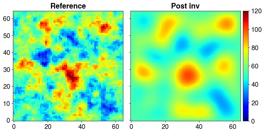
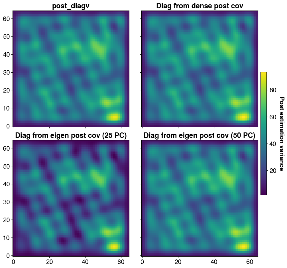
The solver returns an estimate of the posterior variance in the form of a vector of size Ns, which we store here in the variable post_diagv. It is also possible to obtain a low-rank approximation of the posterior covariance matrix. The number of principal components, as well as certain parameters such as inflation, can be adjusted if needed. In this case, we construct the matrix using 25 and then 50 principal components to compare their effects. We also build the full (dense) matrix—although this is not feasible for large-scale problems—for comparison purposes.
post_cov_dense = solver.get_dense_post_cov()
post_cov_25_pc = solver.get_eigen_post_cov(n_pc=25)
post_cov_50_pc = solver.get_eigen_post_cov(n_pc=50)
INFO:PCGA:Preconditioner construction using Generalized Eigen-decomposition
INFO:PCGA:Time for data covarance construction :4.74e-02 sec
INFO:PCGA:Preconditioner construction using Generalized Eigen-decomposition
INFO:PCGA:Time for data covarance construction :2.42e-02 sec
INFO:PCGA:Preconditioner construction using Generalized Eigen-decomposition
INFO:PCGA:Time for data covarance construction :2.82e-02 secAs previously, the higher the number of PC, the better the approximation of the posterior variance
plotter = ngp.Plotter(
    plt.figure(figsize=(10.0, 9.3), constrained_layout=True),
    builder=ngp.SubplotsMosaicBuilder([["diag", "dense"],["25pc", "50pc"]]),
)

ngp.multi_imshow(
    plotter.axes,
    data={
        "post_diagv": post_diagv.reshape(nx, ny, order="F").T,
        "Diag from dense post cov": np.diagonal(post_cov_dense).reshape(nx, ny, order="F").T,
        "Diag from eigen post cov (25 PC)": post_cov_25_pc.get_diagonal()
        .reshape(nx, ny, order="F")
        .T,
        "Diag from eigen post cov (50 PC)": post_cov_50_pc.get_diagonal()
        .reshape(nx, ny, order="F")
        .T,
    },
    fig=plotter.fig,
    imshow_kwargs=dict(
        origin="lower",
        cmap=plt.get_cmap("viridis"),
        aspect="equal",
    ),
    cbar_kwargs=dict(pad=0.01, shrink=0.5),
    cbar_title="Post estimation variance"
)
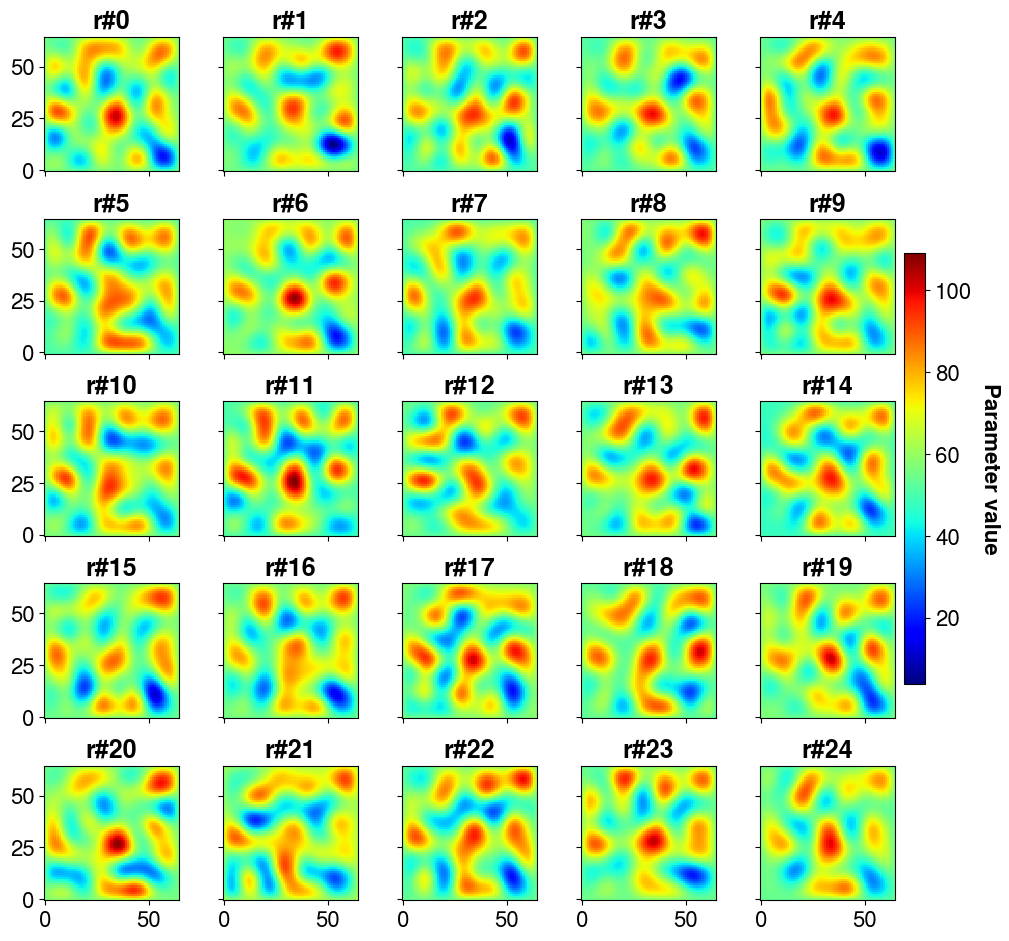
The interest of having the posterior covariance matrix (of inversed parameter values) is that it is possible to draw samples (realizations) from it and thus quantify the uncertainty on predictions (at the cost of one forward call per sample)
# make 200 posterior realizations => we sample from post_cov_50_pc and add the results to s_hat, our inversed parameter vector
post_samples = (
    s_hat.T
    + post_cov_50_pc.sample_mvnormal(shape=(200,), random_state=solver.random_state)
).T
post_samples.shape
(4225, 200)Let’s plot the first 25 realizations
nrows = 5
ncols = 5
plotter = ngp.Plotter(
    plt.figure(figsize=(10.0, 9.3), constrained_layout=True),
    builder=ngp.SubplotsMosaicBuilder(
        [[f"ax{i}-{j}" for i in range(nrows)] for j in range(ncols)],
        sharex=True,
        sharey=True,
    ),
)

ngp.multi_imshow(
    plotter.axes,
    data={
        f"r#{i}": post_samples[:, i].reshape(nx, ny, order="F").T
        for i in range(nrows * ncols)
    },
    fig=plotter.fig,
    imshow_kwargs=dict(
        origin="lower",
        cmap=plt.get_cmap("jet"),
        aspect="equal",
    ),
    cbar_kwargs=dict(pad=0.01, shrink=0.5),
    cbar_title="Parameter value",
)
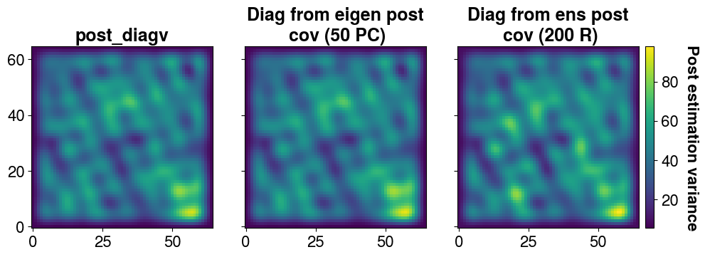
It is possible to find the variance back from the ensemble
# Covariance from the ensemble
post_cov_ens = covmats.CovViaEnsemble(post_samples.T)

plotter = ngp.Plotter(
    plt.figure(figsize=(10.0, 3.5), constrained_layout=True),
    builder=ngp.SubplotsMosaicBuilder([["diag", "50pc", "ens"]]),
)

ngp.multi_imshow(
    plotter.axes,
    data={
        "post_diagv": post_diagv.reshape(nx, ny, order="F").T,
        "Diag from eigen post\n cov (50 PC)": post_cov_50_pc.get_diagonal()
        .reshape(nx, ny, order="F").T,
        "Diag from ens post\n cov (200 R)": post_cov_ens.get_diagonal()
        .reshape(nx, ny, order="F")
        .T,
    },
    fig=plotter.fig,
    imshow_kwargs=dict(
        origin="lower",
        cmap=plt.get_cmap("viridis"),
        aspect="equal",
    ),
    cbar_kwargs=dict(pad=0.01),
    cbar_title="Post estimation variance"
)
📚 Main References
J Lee, H Yoon, PK Kitanidis, CJ Werth, AJ Valocchi, “Scalable subsurface inverse modeling of huge data sets with an application to tracer concentration breakthrough data from magnetic resonance imaging”, Water Resources Research 52 (7), 5213-5231
AK Saibaba, J Lee, PK Kitanidis, Randomized algorithms for generalized Hermitian eigenvalue problems with application to computing Karhunen–Loève expansion, Numerical Linear Algebra with Applications 23 (2), 314-339
J Lee, PK Kitanidis, “Large‐scale hydraulic tomography and joint inversion of head and tracer data using the Principal Component Geostatistical Approach (PCGA)”, WRR 50 (7), 5410-5427
PK Kitanidis, J Lee, Principal Component Geostatistical Approach for large‐dimensional inverse problems, WRR 50 (7), 5428-5443
📌 Applications
T. Kadeethum, D. O’Malley, JN Fuhg, Y. Choi, J. Lee, HS Viswanathan and N. Bouklas, A framework for data-driven solution and parameter estimation of PDEs using conditional generative adversarial networks, Nature Computational Science, 819–829, 2021
J Lee, H Ghorbanidehno, M Farthing, T. Hesser, EF Darve, and PK Kitanidis, Riverine bathymetry imaging with indirect observations, Water Resources Research, 54(5): 3704-3727, 2018
J Lee, A Kokkinaki, PK Kitanidis, Fast large-scale joint inversion for deep aquifer characterization using pressure and heat tracer measurements, Transport in Porous Media, 123(3): 533-543, 2018
PK Kang, J Lee, X Fu, S Lee, PK Kitanidis, J Ruben, Improved Characterization of Heterogeneous Permeability in Saline Aquifers from Transient Pressure Data during Freshwater Injection, Water Resources Research, 53(5): 4444-458, 2017
S. Fakhreddine, J Lee, PK Kitanidis, S Fendorf, M Rolle, Imaging Geochemical Heterogeneities Using Inverse Reactive Transport Modeling: an Example Relevant for Characterizing Arsenic Mobilization and Distribution, Advances in Water Resources, 88: 186-197, 2016
📝 Credits
pypcga is based on Lee et al. [2016] and currently used for Stanford-USACE ERDC project led by EF Darve and PK Kitanidis and NSF EPSCoR Ike Wai project.
Code contributors include:
🔑 License
This project is released under the BSD 3-Clause License.
Copyright (c) 2018-2026, Jonghyun Lee. All rights reserved.
For more details, see the LICENSE file included in this repository.
⚠️ Disclaimer
This software is provided “as is”, without warranty of any kind, express or implied, including but not limited to the warranties of merchantability, fitness for a particular purpose, or non-infringement. In no event shall the authors or copyright holders be liable for any claim, damages, or other liability, whether in an action of contract, tort, or otherwise, arising from, out of, or in connection with the software or the use or other dealings in the software.
By using this software, you agree to accept full responsibility for any consequences, and you waive any claims against the authors or contributors.
📧 Contact
For questions, suggestions, or contributions, you can reach out via:
We welcome contributions!
Free software: SPDX-License-Identifier: BSD-3-Clause
Project details
Release history Release notifications | RSS feed

Download files
Download the file for your platform. If you're not sure which to choose, learn more about installing packages.
Source Distribution
Built Distribution
Filter files by name, interpreter, ABI, and platform.
If you're not sure about the file name format, learn more about wheel file names.
Copy a direct link to the current filters
File details
Details for the file pypcga-0.2.0.tar.gz.
File metadata
- Download URL: pypcga-0.2.0.tar.gz
- Upload date:
- Size: 53.6 kB
- Tags: Source
- Uploaded using Trusted Publishing? No
- Uploaded via: twine/6.2.0 CPython/3.13.11
File hashes
| Algorithm | Hash digest | |
|---|---|---|
| SHA256 |
88f3401e421ff0c645d0c4136fa6354a33e56cb9011980290864b3322503dffd
|
|
| MD5 |
515779bf408a1a572bc8021f98c134ae
|
|
| BLAKE2b-256 |
5f6910ab12439d1c29ff54745e3acf912bdf571a61e13dfffc58abdd152d1482
|
File details
Details for the file pypcga-0.2.0-py3-none-any.whl.
File metadata
- Download URL: pypcga-0.2.0-py3-none-any.whl
- Upload date:
- Size: 33.0 kB
- Tags: Python 3
- Uploaded using Trusted Publishing? No
- Uploaded via: twine/6.2.0 CPython/3.13.11
File hashes
| Algorithm | Hash digest | |
|---|---|---|
| SHA256 |
f21b3e95b7a86b80fff7450e0c2a4d9a6910d4cc441c4825d8c9cf16789dadc5
|
|
| MD5 |
22d27f2f79732aa12ec129c7bdbaf60e
|
|
| BLAKE2b-256 |
8ece835d60c43a9f923b75abd197ada665f8bc113291e38892261942a20d7b11
|


