
This release is a pre-release and may not be stable for production use.
pyplatypus

Computer vision for medical imaging — the engine behind the platypus R package.
An alpha. This replaces the 2022 TensorFlow package with a PyTorch one, and the API still moves, so pin the exact version if you build on it. The changelog says what each release changed; no version number is repeated here, because the one that was went four releases stale.
Everything on PyPI so far is a pre-release, so
pip install pyplatypusresolves to the newest.pip install pyplatypus==0.1.0rc2gets the old TensorFlow package.
Most people should reach this through rplatypus, the R package: it installs this one, calls it, and is where the worked examples and the plotting live. Use it directly if you are writing Python.
The two have one documentation site each, built the same way, with the same sections in the same order - and one configuration format, because it is the same file read by the same models whichever language asked.
Installing
Python ≥ 3.10, and torch ≥ 2.7.
To fetch published weights by name, install the hub extra:
pip install "pyplatypus[hub]"
It is not in the base install because most runs never fetch weights and an air-gapped one cannot. Local weights files and everything else work without it.
For a pretrained encoder, install the encoders extra, which brings timm:
pip install "pyplatypus[encoders]"
On a Pascal-generation GPU ask for both extras together — pyplatypus[encoders,pascal]. timm
pulls in torchvision, torchvision pins its torch version by equality, and asking for timm alone
resolved torch to a CUDA 13 build whose kernels start at sm_75; a GTX 1070 is sm_61, so the
GPU disappears and the error blames the driver. The two extras together resolve to torch 2.7.1
and torchvision 0.22.1.
If your GPU is a GTX 10-series (Pascal) or older, install the pascal extra:
pip install "pyplatypus[pascal]"
torch 2.8 and later ship CUDA 13 builds, and CUDA 13 dropped the Maxwell, Pascal and Volta generations outright - no driver update brings them back. The last torch built against CUDA 12 is 2.7.x, which the extra pins. On anything from Turing (RTX 20-series) onwards, ignore this.
A worked example
uv venv --python 3.11 .venv
uv pip install --python .venv/bin/python -e ".[dev]"
.venv/bin/python -m pytest

# The linter is pinned in pyproject.toml and installed on its own, so it agrees with CI
# and does not drag torch along to read text files.
uv run --only-group lint ruff check pyplatypus tests
from pyplatypus import build_engine, from_yaml

engine = build_engine(from_yaml("examples/data_science_bowl.yaml"))
engine.fit(verbose=True)

for row in engine.evaluate():
    print(row)

masks = engine.predict(engine.best_model("dice"), split="test")
examples/data_science_bowl.yaml trains a U-Net and a LinkNet on the 2018 Data Science
Bowl and prints a comparison. On a GTX 1070 that is about 11 seconds per epoch at
160×160.
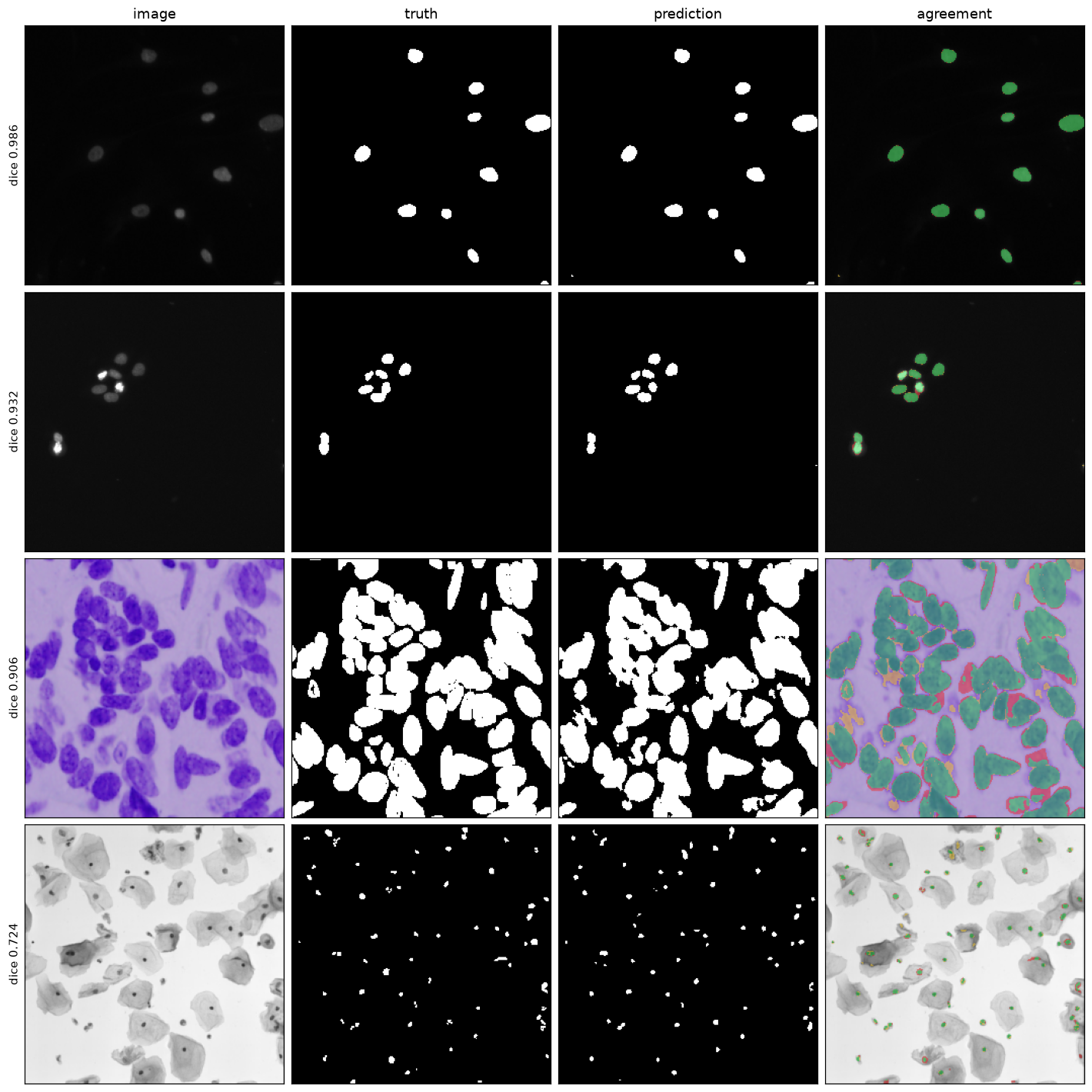
Four of the 134 images dsbowl-unet was held out from, drawn by plot_masks() here - the
best, two from the middle of the ranking and the worst, so the picture covers the
distribution the model card reports rather than its top. Green is what was found, red what
was missed, yellow what was invented.
The bottom row is the card's worst case at 0.724 and it shows what that number is: tiny dark
nuclei in a brightfield image, where the model finds specks. Dice for the whole split comes
back as 0.9205, which is the card's own figure to four decimals - tools/readme_figures.py
remakes the seeded split the weights were measured on and refuses to draw if the cases the
card names are not in it.
The same thing from a file
The point of a specification holding several models is that the comparison costs one command. Run
examples/compare_dsbowl_architectures.py and all four architectures train on the same split with
the same augmentation:
| model | parameters | s/epoch | epochs | Dice mean | sd | median | min |
|---|---|---|---|---|---|---|---|
| U-Net | 1,942,594 | 15.5 | 60 | 0.9217 | 0.054 | 0.9353 | 0.7227 |
| U-Net++ | 2,263,730 | 18.8 | 44 | 0.9212 | 0.055 | 0.9323 | 0.7459 |
| LinkNet | 1,746,754 | 14.0 | 60 | 0.9203 | 0.053 | 0.9293 | 0.7205 |
| Res-U-Net | 2,029,682 | 14.2 | 55 | 0.9187 | 0.058 | 0.9293 | 0.6706 |
Which is worth reading for what it says rather than for the winner. The spread across the four is 0.0030, and the spread across images within any one of them is 0.054 — the architectures are eighteen times closer to each other than the images are. Re-running the same U-Net with a different seed moves the number by 0.0012, which is 40% of the whole spread.
On this problem the architecture is not where the result comes from, and a table like this is how you find that out in an hour instead of a fortnight. That is also why only one set of weights is published: four names that mean the same thing would be four promises nobody needed.
What is in it
Semantic segmentation in 2D, end to end:
- One spec, two ways in. Build it from arguments or load it from YAML — both produce the same object, so nothing downstream can tell which you used.
- Four architectures: U-Net, U-Net++, Res-U-Net, LinkNet, each composable with separable convolutions, spatial dropout, learned or interpolated upsampling, deep supervision and configurable block width.
- Nine losses (IoU, Dice, CCE, CCE-Dice, Focal, Tversky, Focal-Tversky, Combo, Lovász) and three metrics, all reducing over every axis except batch and channel — so they already work on volumes.
- Instances, and what they are worth:
task: instance_segmentationkeeps the per-object masks apart instead of uniting them, derives the head's width from aseparation:block namedrimorflows, and scores the Data Science Bowl's own average precision after a post-process.decode:is a list, because several decodings share one forward pass - a second one costs 1.41 s against 16 minutes for a second training run - soevaluate()returns a row per (model, decoding) withconnected_componentsalways among them. Read that row first: it ignores the separation signal, and a perfect semantic mask scores 0.7655 through it on this data, because touching nuclei are one region. The signal itself is worth +0.068 at best where a perfect mask is worth +0.2398 - measured, three ways, and the reason that number is here rather than in a footnote. - Tiling that goes both ways: cut a large image into a grid instead of shrinking it, and get a full-size mask back.
- DICOM, read properly: stored values converted to real units through the modality LUT, a fixed window rather than one taken from the image, and MONOCHROME1 inverted. Opening the file is the easy part; those three are what make two scans comparable.
- Splitting by patient, not by slice:
split_dataset()turns one directory into train/validation/test CSVs, keeping every group whole. Slices of one patient on both sides of a split is the most common way to publish a Dice that means nothing, and agroup_bythat matches nothing is an error rather than a silent fallback. - Scores per case, not one number:
evaluate_cases()reports each image or patient separately andsummarise_cases()gives the distribution and names the worst one. On the Data Science Bowl a model at 0.855 over the split turned out to score 0.006 on three images; the mean had no way of saying so. - Volumes, not only slices: NIfTI in, 3D U-Net out, patches through the same tiling
that cuts 2D images. Every volume is reoriented to canonical (RAS) first - a NIfTI's
affine, not its array order, says where the anatomy is, and two datasets read naively can
be mirror images of each other. Masks may be label maps (
labels: [0, 1]) as well as pictures, because that is how every volume format stores them. - Resampling to a common voxel size:
target_spacing: [1, 1, 1]fixes the millimetres per voxel and then centre-crops or pads to the model'sinput_shape, instead of squeezing every scan into the same box. Clinical scans cover whatever length the question needed - 40 slices of 1 mm is 40 mm of patient, 40 slices of 2.5 mm is 100 mm - so resizing alone makes the same organ a different size in each and the network cannot tell. - One channel per file, in a stated order:
channels_fromtakes one pattern per channel, which is how BraTS ships four MRI sequences per patient and how satellite sets keep their bands. Sorting the names gives flair, t1, t1ce, t2 - reproducible, and anatomically meaningless; a model trained with FLAIR in channel one and used where channel one is T1 answers plausibly and reports nothing. A pattern matching two files, or none, or leaving a file unused, is an error. - The answer on the grid it came from:
predict(space="source")maps each prediction back onto the scan it was computed from, undoing the resampling and the crop. A mask on the model's grid cannot be laid over the patient's scan by anything, which is the whole point of producing one. Returns a list rather than an array, because scans differ in size and resizing them to match is how a mask ends up describing the wrong anatomy. - Weights by name, pinned to a commit:
weights: dsbowl-unetis published and fetches from a registry entry that carries the exact commit they were published at, so a name means one set of numbers forever.hf://owner/repo/file.safetensors@committakes anything else on the Hub, a path takes a local file, and a sidecar records what the weights were trained for - loading refuses a model they do not belong to, because weights with the wrong colormap and the right shape load cleanly and predict nonsense. - A refusal before training on masks the colormap does not describe. This is the
quietest way a segmentation run wastes a day: the colours in the specification match none of
the labelled tissue, every mask reads as background, the loss falls because background is
most of a medical image, and the model learns to answer "nothing here".
fit()now reads a sample of the training masks first and refuses when a declared class appears in none of them - which is provable rather than suspicious, since a class with no examples has no gradient towards it. It also refuseslabelsthat leave out 0 when any voxel matches none of them, because index 0 is both the first entry of a naming and where an unmatched voxel goes - so without it the background trains as a real class and the target stays plausible while it happens.Engine(..., check_masks=False)proceeds anyway. - Many models from one file, with a comparison table at the end - which is how you find out that on some problems the architecture is not what matters. See below.
- A pretrained backbone as the contracting path:
encoder: resnet34builds that architecture, andpretrained: trueis the separate flag that loads its ImageNet weights - separate because the first thing a named backbone should not do is reach the network on a machine that has none. Any timm backbone whose features start at half resolution works;blockssays how many of its stages to use, and the full-resolution level a U-shaped decoder needs is one block of ours, because no ImageNet stem has one. What it is measurably worth, and what it is not, is below.
Augmentation works in 3D, with a caveat the package handles rather than hides: albumentations
supports volumes unevenly - most of its transforms take one and the rest raise from inside the
library, GaussNoise as KeyError: 'images'. The count is deliberately not written here: it
is the outcome of probing the installed version, and one CI matrix answered two different
numbers on the same albumentations. Every transform in a 3D specification is tried against a
probe volume while the pipeline is built, so an unsupported one is named before training
starts, and available_transforms(rank=3) lists what is usable.
Resampling is opt-in rather than automatic: it changes the voxel grid the model sees, which
is a decision to take deliberately. Without target_spacing the old behaviour stands and
volumes are resized to input_shape.
Boxes instead of masks
task: object_detection in a specification gives a YOLOv3 trained from the same pipeline -
anchors fitted to your own boxes, Pascal VOC or LabelMe annotations, predictions back in each
image's own pixels, and mean average precision per class that agrees with pycocotools. On
BCCD, from nothing, over five seeds:
mAP@0.5                    0.8660 +/- 0.0159
mAP@[.50:.95]              0.5159 +/- 0.0199
mean IoU of matched boxes  0.8041 +/- 0.0026
about 37 minutes a seed on a GTX 1070, and examples/detect_blood_cells.py is that run.
Five seeds rather than one, because on this dataset a single number would be whichever seed got reported: the runs span 0.853 to 0.887 of mAP@0.5. How well the boxes fit is far steadier than how many are found - the matched overlap varies by a quarter of a point where average precision varies by one and a half - so a difference of a point in mAP here is not a result, and the first draft of this work read several of them as one.
bccd-yolo3 is published, so boxes on an image need no GPU and no afternoon:
engine = build_engine(from_dict({
    "task": "object_detection",
    "data": {"train_path": "images/", "validation_path": "images/",
             "classes": ["RBC", "WBC", "Platelets"]},
    "models": [{"name": "cells", "input_shape": [416, 416],
                "weights": "bccd-yolo3", "fit": False}],
}))
engine.fit()                               # loads the weights, trains nothing
found = engine.predict("cells", "validation")
The anchors come out of the sidecar beside the file and are adopted, because a detector's
weights mean nothing without them - read with any others they give plausible boxes in the
wrong places. A specification that names its own anchors alongside weights is refused
rather than quietly overruled.
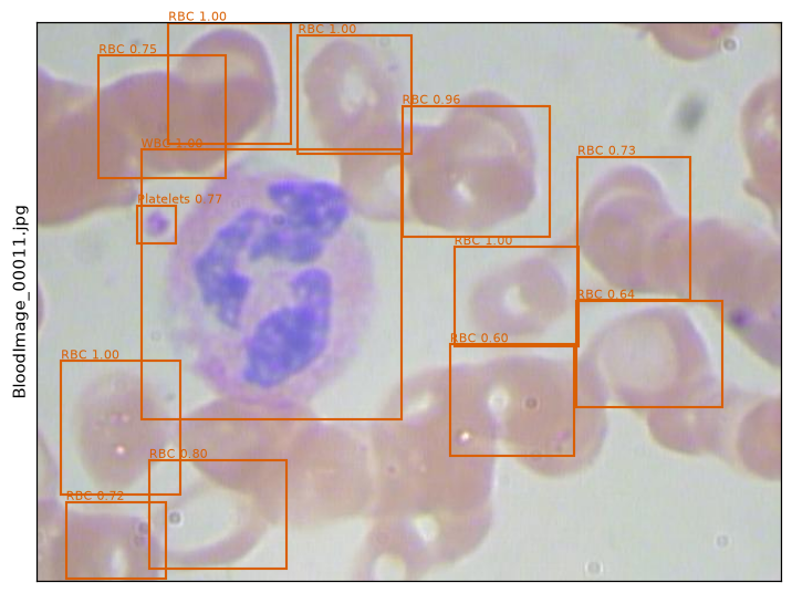
One frame of BCCD's held-out split, drawn by bccd-yolo3 - published with these packages, so
the picture costs a download rather than an afternoon. The frame is chosen by reading the
annotations rather than by eye, because a picture of red cells alone shows a third of what the
detector does: both rare classes are here, the white cell at 1.00 and the platelet at 0.77.
Eleven red cells are drawn at a threshold of 0.5 where seventeen are annotated.
plot_boxes() takes what predict() returns with nothing rearranged in between. The R
package draws the same frame, from the same weights, through ggplot2 rather than matplotlib,
and finds the same eleven boxes at the same scores.
A backbone instead of the built-in encoder
encoder and pretrained are two flags, not one, and the reason is that the second is the only
one that reaches the network:
models:
  - name: polyps
    encoder: resnet34        # builds a ResNet-34 contracting path
    pretrained: true         # and loads its ImageNet weights
    freeze_encoder: 5        # holding them still while the decoder settles
Measured on three datasets, one per modality, 3 seeds each, each configuration compared at its best validation Dice with the best weights restored. Small training sets on purpose - 40 to 100 images - because that is the regime transfer learning is supposed to be for.
| DS Bowl, microscopy | SIIM-ACR, chest X-ray | Kvasir-SEG, endoscopy | |
|---|---|---|---|
| built-in encoder, 1.9M | 0.8460 ±0.0068 | 0.0531 ±0.0586 | 0.5830 ±0.0128 |
| resnet34 from scratch, 9.0M | 0.7891 ±0.0992 | 0.1073 ±0.0033 | 0.5670 ±0.0251 |
pretrained, freeze_encoder: 5 |
0.8333 ±0.0151 | 0.1203 ±0.0116 | 0.5932 ±0.0170 |
pretrained, encoder_learning_rate: lr/10 |
0.8326 ±0.0094 | 0.1011 ±0.0092 | 0.5329 ±0.0101 |
Four things come out of it, and they repeat on all three:
Use freeze_encoder, not encoder_learning_rate alone. Freezing is the better pretrained
variant everywhere, and on Kvasir a tenth of the learning rate is the worst configuration in the
table - below the built-in encoder and below the same ResNet trained from nothing. Giving one
learning rate to the whole network is worse still: on DS Bowl it costs 0.045 of Dice and
quadruples the seed spread, because a random decoder's gradients undo the transferred weights
before the decoder has learned anything to be worth it.
Do not expect a better score. Expect to reach it sooner. On Kvasir the built-in encoder needed 150, 110 and 83 epochs for its three seeds; pretrained-and-frozen needed 64, 82 and 83 for the same Dice. That halving is the one benefit that showed up consistently.
Capacity matters where the target is thin. On SIIM, where a pneumothorax covers a median 0.59% of the frame, every ResNet variant roughly doubles the built-in encoder's score - and the built-in encoder's seed spread (±0.0586) is larger than its own mean, with two of three seeds never learning at all. That is an argument for being able to swap the encoder, independent of ImageNet.
ImageNet features do not transfer to these images. The clearest number is from DS Bowl with the backbone frozen for the whole run: 0.6068, against 0.8460 for an encoder that learned the task from 40 images. And Kvasir is the fairest test available - camera photographs of tissue, three channels, natural lighting - where the best pretrained configuration beats the built-in encoder by 0.0102 with a seed spread of 0.0170. Inside the noise.
So the feature is here, correct, and documented for what it does: a faster route to the same answer, and a bigger encoder for problems that need one. Our own 1.9M-parameter encoder beats ResNet-34's 9.0M on two of the three datasets.
Reproduce with examples/compare_pretrained_encoders.py. Raw logs and per-seed numbers are in
measurements/. The SIIM-ACR images came from a Kaggle competition, so no weights trained on
them are published; BBBC038v1 is CC0 and Kvasir-SEG is CC BY 4.0.
Learning it
The documentation site carries three things, and which one you want depends on the question:
-
Writing a configuration walks from one model to several - the required fields, comparing variants in one run, dividing a folder by patient, detection, published weights, and what is checked when.
-
Every configuration field is generated from the schema the models produce, so it cannot describe a field this package does not have. Point your editor at it and it will check a file as you type:
# yaml-language-server: $schema=https://maju116.github.io/pyplatypus/schema/spec.schema.json -
The reference is generated from the docstrings, and the
>>>examples in them are run bypytest --doctest-modules- so the site cannot show an example that does not work.
examples/ holds the programs the measurements on this page came from, which is the other
way to read it: every table here is reproducible by running the script named beside it.
The R package's vignettes are worked examples on real datasets, listed on that page, and the pipeline underneath is this one - so they are worth reading even if you never write R.
What is not in it yet
Ensembling remains out of scope.
Multilabel segmentation - a voxel belonging to two classes at once - is not here either, and
it is structural rather than a missing flag: the output is a softmax over channels and both
mask representations encode one class per voxel. MULTILABEL_RECON.md measures what it would
take and
pyplatypus#91 is where the first decision
sits.
Classification has no task of its own. DetectionEngine.crops() cuts detected objects out of
their images at a fixed size, which is the half of it this package is the right place for; the
classifier is yours.
About the author

Both halves of this are by Michał Maj — this Python package, and the R package it is reached from.
The first version was a Keras and TensorFlow package in 2020, and it is still on master
with the stars and the open issues it earned. Everything here was written from scratch in
2026 on torch, which is why the version numbers restart rather than continue.
Licence
MIT.
1 maintainer

Metadata
1 maintainer
Release files for pyplatypus 0.8.0a29
For a detailed explanation of source distributions (sdists) and built distributions (wheels), please see the package formats documentation.
Source distribution (sdist)
| File | Size | Uploaded | Provenance | |
|---|---|---|---|---|
| pyplatypus-0.8.0a29.tar.gz | 682.1 kB | With provenance | Details |
Built distribution (wheel)
| File | Interpreter | ABI | Platform | Reset |
|---|---|---|---|---|
| pyplatypus-0.8.0a29-py3-none-any.whl | Python 3 | none | any | Details |
Total release size: 1.0 MB
Release files / pyplatypus-0.8.0a29.tar.gz
| Download URL | pyplatypus-0.8.0a29.tar.gz |
|---|---|
| Size | 682.1 kB |
| Tags | Source |
|
SHA-256 checksum How to use checksums |
aac7b118a64c939ac9146bc1fac4361bdf697ac82f30f9eadabb4be1a7e13e02
|
|
BLAKE2b-256 checksum How to use checksums |
c89b26bbcb31a9d2209f0fa538df73761b2817d793bd52e34508d4d83def5b83
|
| Upload date | |
|
Uploaded using Trusted Publishing? What is trusted publishing? |
Yes |
| Uploaded via |
twine/7.0.0 CPython/3.13.16
|
Provenance
Provenance describes where a file came from. On PyPI, provenance is shared via attestations, which provide a verifiable record of the build or publishing details. View details, limitations and caveats.


PyPI Publish Attestation
PyPI verified that this artifact, at this checksum, originated from the publisher listed below.
Signed by GitHub Actions, verified by PyPI on Oct 23, 2026.
Transparency logRelease files / pyplatypus-0.8.0a29-py3-none-any.whl
| Download URL | pyplatypus-0.8.0a29-py3-none-any.whl |
|---|---|
| Size | 343.4 kB |
| Tags | Python 3 |
|
SHA-256 checksum How to use checksums |
885d973e4d68a6a85d4ee19c1d66e66af3f350121c99389310bfb2ea1336dbb7
|
|
BLAKE2b-256 checksum How to use checksums |
7e96c64d03fc7b200886664bb1f948aa45f00c8c0797755eb68affa78cd60682
|
| Upload date | |
|
Uploaded using Trusted Publishing? What is trusted publishing? |
Yes |
| Uploaded via |
twine/7.0.0 CPython/3.13.16
|
Provenance
Provenance describes where a file came from. On PyPI, provenance is shared via attestations, which provide a verifiable record of the build or publishing details. View details, limitations and caveats.
PyPI Publish Attestation
PyPI verified that this artifact, at this checksum, originated from the publisher listed below.
Signed by GitHub Actions, verified by PyPI on Oct 23, 2026.
Transparency logSecurity for pyplatypus 0.8.0a29
Provenance
Provenance describes where a file came from. On PyPI, provenance is shared via attestations, which provide a verifiable record of the build or publishing details. View details, limitations and caveats.
Full provenance
All 2 files in this release have been uploaded with provenance metadata.
Attestation for pyplatypus-0.8.0a29.tar.gz
PyPI Publish Attestation
PyPI verified that this artifact, at this checksum, originated from the publisher listed below.
Signed by GitHub Actions, verified by PyPI on Oct 23, 2026.
Transparency logA note on package security
PyPI is a repository for distributing packages, not a service for auditing them. While third-party security researchers and our staff do their best to detect and remove malicious packages, PyPI cannot guarantee the quality, security or suitability of any given package.
To learn more about protecting yourself from malicious actors, visit our package security documentation.














