
pyshindo




概要
pyshindo は加速度から気象庁の計測震度を計算するPythonパッケージです。記録全体を使うFFT参照計算(計測震度)と、逐次入力向けの因果的リアルタイム近似を明確に分離しているのが特徴です。気象庁の公開計算式、Kunugi et al. (2008, 2013)、および関連特許(JP4229337B2 / JP5946067B2 / JP7681907B2)に基づき、係数は固定表を転記するのではなく式から都度導出しています。リアルタイム側は直近60秒の閾値をヒストグラム丸めなしの厳密な順序統計量で保持し、逐次入力(process_sample)と一括入力(process)のどちらでも同じ結果になるよう作られています。
計測震度に加えて、長周期地震動階級、PGV・PGD(最大速度・最大変位。いずれも気象庁が定義・公表している量です)、SI値(Housnerのスペクトル強度)も算出できます。長周期地震動階級は気象庁が公開している絶対速度応答スペクトルと照合し、2地震・268観測点で全ての階級が一致、応答スペクトル自体も最大値で1e-05程度、検証した観測点のうち最も悪いところで1.7e-05の水準で一致することを確認しています。ObsPy連携を使えば、K-NET・KiK-net・miniSEED・SACなどObsPyが読める形式をそのまま入力にできます。
詳細なアルゴリズム解説は日本語で docs/algorithm.md(計測震度)と docs/long-period.md(長周期地震動階級)にあります。
本パッケージは個人で開発しているものです。一次資料にあたって実装し、公開データとの照合結果もdocs/validation.mdに記録していますが、計算結果の正確性・完全性を保証するものではありません。ご利用は自己判断・自己責任でお願いします。
pyshindo is a small Python package for calculating Japanese instrumental seismic intensity from acceleration records. It keeps the complete-record FFT calculation separate from causal real-time approximations, so the meaning of both results remains explicit.
The package targets Python 3.12 or later. It is a research and engineering reference implementation, not a certified seismic intensity meter, earthquake early-warning service, or safety controller.
What is implemented
- The published JMA frequency-domain calculation: FFT per component, the three-factor intensity response, inverse FFT, three-component resultant, the 0.3-second cumulative-duration threshold, and the official decimal treatment.
- The original 2008 causal approximation filter.
- The improved 2012 causal approximation filter.
- The generalized low-sampling-rate filter disclosed in JP7681907B2.
- Exact rolling order statistics for a 60-second real-time window without discretizing intensity into fixed-width bins.
- Stateful chunk and single-sample APIs whose results are invariant to chunk boundaries.
- Unit conversion, sampling diagnostics, PGA, preprocessing helpers, JMA text-record parsing, and optional Plotly figures.
- Velocity and displacement by cumulative trapezoidal integration, and PGV/PGD -- with the baseline treatment left to the caller rather than applied silently. Displacement compounds the same drift a second time, so it is considerably more baseline-sensitive than velocity.
- The JMA long-period ground motion class (長周期地震動階級): the 20-second high-pass, a 32-oscillator bank over 1.6-7.8 s, the horizontal vector composite, the overall and per-band classes, and a streaming estimator. Every class matches JMA's own published values across 268 stations of two earthquakes; the response spectra themselves agree to about 1e-5, worst case, over the stations checked.
- Housner's spectrum intensity (SI value), per component: the relative-velocity response spectrum averaged over the 0.1-2.5 s period band, sharing the same linear-acceleration-method oscillator solver as the long-period class but without its absolute-velocity or component-combination steps, plus a streaming estimator with the same cumulative-maximum behavior as the long-period class's.
- A general elastic response spectrum (
calculate_response_spectrum): relative displacement, relative velocity, pseudo-velocity, and pseudo-acceleration for any damping ratio and period grid, sharing the same oscillator solver as the long-period class and SI value without either one's own conventions baked in. detect_clipping: a diagnostic-only check for saturated samples, by a known digitizer range and/or a run of repeated values near a component's own peak. Never applied automatically.- Optional ObsPy interoperability (
pyshindo[obspy]): convert a stream that ObsPy already read -- K-NET, KiK-net, miniSEED, SAC -- into the arrays used here, without reimplementing any reader. - Each causal filter's named analog factors (
RecursiveFilterDesign.stages) can be inspected or plotted individually, not just as a combined response. - Built-in wall-clock timing: every result carries a
timingfield (or, forprocess_sample,elapsed_s) measured withtime.perf_counter, so callers can inspect calculation cost without wrapping their own timer.
Relevant real-time algorithms are associated with patent documents. Read PATENTS.md before distribution or operational use. The MIT license covers copyright in this source code and is not a patent-clearance opinion.
Separately: Japan's forecasting-business licence (気象業務法 Article 17) covers predicting ground motion before it happens and announcing that prediction, which is a different activity from what this package does -- computing intensity or long-period class after the fact from an already-recorded waveform (overview, in Japanese). Where the line falls in a given use case is not something this note can settle, so it is not legal advice.
Installation
python -m pip install pyshindo
The optional extras are plot for the Plotly figures and obspy for reading
formats through ObsPy:
python -m pip install "pyshindo[plot,obspy]"
For the unreleased state of main, or from a local checkout:
python -m pip install git+https://github.com/aldichollow/pyshindo.git
# from a checkout, editable, with the extras:
python -m pip install -e ".[plot,obspy]"
Complete-record FFT calculation
from pyshindo import calculate_measured_intensity

result = calculate_measured_intensity(
    acceleration,              # shape: (samples, 3)
    sampling_rate_hz=100.0,
    unit="m/s^2",
)

print(result.intensity_raw)                 # Unrounded continuous value
print(result.intensity)                     # Official one-decimal treatment
print(result.scale.japanese)                # Example: "5弱"
print(result.threshold_acceleration_gal)    # 0.3-second threshold
print(result.filtered_pga_gal)
print(result.timing.total_s)                # wall-clock time for this call
result.filtered_acceleration_gal, result.resultant_acceleration_gal, the frequency vector, and the applied response are retained by default. Set retain_intermediates=False for lower memory use.
For a scalar-only call:
from pyshindo import measured_intensity

intensity = measured_intensity(acceleration, 100.0, unit="gal")
Real-time calculation
from pyshindo import RealtimeIntensityEstimator

estimator = RealtimeIntensityEstimator(
    sampling_rate_hz=100.0,
    unit="gal",
)

for chunk in acceleration_chunks:
    output = estimator.process(chunk)
    latest = output.intensity_raw[-1]
    print(output.timing.filter_s, output.timing.order_statistic_s)
The estimator filters every sample, preserves recursive state, and maintains the exact 30th-largest value in the latest 60 seconds at 100 Hz. The first valid output appears with sample 30; preceding values are NaN. A zero threshold maps to negative infinity, as required by the logarithmic conversion.
For one complete-record replay:
from pyshindo import calculate_realtime_intensity

trace = calculate_realtime_intensity(acceleration, 100.0, unit="gal")
print(trace.approximate_intensity_raw)
print(trace.approximate_intensity)
Velocity, displacement, PGV, and PGD
from pyshindo import peak_ground_displacement, peak_ground_velocity, remove_offset

pgv = peak_ground_velocity(remove_offset(acceleration), 100.0, unit="gal")
pgd = peak_ground_displacement(remove_offset(acceleration), 100.0, unit="gal")
Velocity comes from cumulative trapezoidal integration and is always returned in
cm/s (kine); displacement integrates that same velocity a second time and is
always returned in cm. Nothing is baseline-corrected on your behalf:
integration cannot distinguish a baseline error from real long-period motion,
so a record with a nonzero mean integrates into a linearly drifting velocity
-- and, one integration further, a quadratically drifting displacement, so
PGD is considerably more sensitive to an uncorrected baseline than PGV is.
Apply remove_offset, detrend_acceleration, or a high-pass filter first,
and say which one you used. See
examples/06_peak_velocity.py.
peak_ground_velocity/peak_ground_displacement take the resultant of
whichever components you pass, the same as peak_ground_acceleration: three
components give the three-component resultant, two horizontals give the
horizontal PGV/PGD.
JMA's own published peak velocity, in the max.csv of a long-period ground
motion observation page, does not match this default -- but does match, to
about 0.01 percent across 268 stations, once the same 20-second high-pass used
for the long-period class is applied to the acceleration first
(pyshindo.long_period.apply_ground_motion_high_pass). See
docs/validation.md for the finding and
docs/api.md for the recipe.
The same max.csv's published peak displacement is not a double integration
at all -- JMA derives it by filtering acceleration through a filter
reproducing the amplitude response of its mechanical 1x strong-motion
seismometer (natural period 6 s, damping 0.55), which is published in
速度波形・変位波形の求め方.
pyshindo.strong_motion.apply_strong_motion_displacement_filter implements
this directly from acceleration (no separate integration step) and reproduces
the published displacement to a median relative error of about 0.15 percent
across the same 268 stations. See docs/validation.md.
Long-period ground motion class
from pyshindo.long_period import calculate_long_period_class

result = calculate_long_period_class(horizontal_acceleration, 100.0, unit="gal")
print(result.long_period_class)   # "0" through "4"
print(result.max_sva_cm_s)        # absolute velocity response maximum, cm/s
print(result.critical_period_s)
for band in result.bands:         # the per-band classes JMA also reports
    print(band.japanese_label, band.long_period_class)
A different quantity from instrumental intensity and a different calculation:
horizontal components only, a bank of damped oscillators covering 1.6 to 7.8
seconds, and the largest absolute velocity response. LongPeriodEstimator
gives the same numbers incrementally for streaming input.
Checked against JMA's own published absolute velocity response spectra: across
268 stations of two earthquakes, every long-period class matches, and the
spectra themselves agree to about 1e-5, worst case among the stations checked.
See docs/long-period.md for the algorithm and its
primary sources, docs/validation.md for the full
comparison, and examples/08_long_period.py to
reproduce it.
Spectrum intensity (SI value)
from pyshindo import calculate_spectrum_intensity

result = calculate_spectrum_intensity(acceleration, 100.0, unit="gal")
print(result.si_cm_s)   # one value per component, not combined
Housner's SI: SI = (1/2.4) * integral[0.1, 2.5] Sv(T, h=0.20) dT, where Sv
is the relative velocity response spectrum -- not the absolute response the
long-period class uses, and not combined across horizontal components,
matching the same choice peak_ground_velocity leaves to the caller. The
oscillator response itself shares the long-period class's linear-acceleration
solver, without its ground-velocity or vector-combination steps.
Neither the damping ratio (0.20, specific to SI, not a general structural
value) nor the 0.1-2.5 s integration range has changed across the sources
checked, but no published discretization exists for evaluating that integral
numerically; the 121-point grid used here was chosen by checking convergence
directly. See examples/09_spectrum_intensity.py.
Reading other formats through ObsPy
import obspy
from pyshindo.obspy_interop import from_obspy_stream

stream = obspy.read("...").select(station="...")
record = from_obspy_stream(stream, unit="gal")
A thin adapter, not a reader: it converts a stream that is already in
acceleration units into the arrays used here and never resamples, trims,
merges, rotates, or rescales. unit is required rather than detected, because
SEED and the formats around it carry no dependable physical-unit field. See
docs/data.md and
examples/07_obspy_interop.py.
Sampling rates other than 100 Hz
The FFT calculation accepts any positive sampling rate and evaluates the published response at the corresponding FFT frequencies. A warning is emitted because comparability still depends on the source bandwidth, anti-aliasing, record preparation, and validation data.
The default real-time selection is RealtimeFilter.AUTO:
- at 80 Hz or above, the improved 2012 filter is used;
- below 80 Hz, the generalized low-rate design is used;
- below 1 Hz, no published gamma table is available and an error is raised.
The selected design is recorded in result.filter_name. An explicit 2012 request is checked for pole stability and fails instead of returning a diverging sequence. Batch resampling is available through resample_acceleration, but is never performed implicitly.
Data and figures
pyshindo.io parses the seven-line JMA strong-motion text header and can download one explicitly selected URL. No observed waveform is bundled. See docs/data.md.
Plotly figures use a restrained package theme. Intensity colors 1 through 7 follow the JMA web color guide; the guide does not assign intensity 0 a color, so the neutral intensity-0 background is identified as a package choice. The long-period class colors are the ones JMA uses on its own long-period observation pages. Multi-station distribution maps (intensity_map_figure, long_period_class_map_figure, continuous_value_map_figure) share the same colors, taking parallel latitude/longitude/value arrays from whichever source produced them.
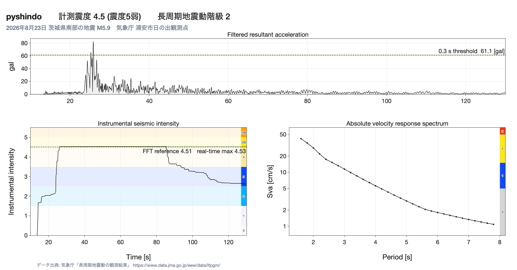
1つの実記録から計算した例。2026年8月23日 茨城県南部の地震 M5.9、気象庁 浦安市日の出観測点。 上段は0.3秒継続の閾値がどこで選ばれるか、左下は同じ記録に対するリアルタイム近似とFFT参照計算がほぼ一致すること、 右下は長周期地震動階級を示しています。データ出典: 気象庁「長周期地震動の観測結果」。
Documentation
- Algorithm guide (Japanese)
- API reference (Japanese)
- Long-period ground motion class (Japanese)
- Observed data I/O (Japanese)
- Validation against JMA's published values (Japanese)
- Migration guide (Japanese)
Examples
Each file in examples/ is a runnable script written with # %%
cell markers, so it can be executed top to bottom or stepped through in an
interactive window.
00_quickstart.py |
Every headline result in one page: measured intensity, real-time intensity, PGV/PGD, long-period class, SI value |
01_measured_intensity.py |
The FFT reference calculation and its intermediate waveforms |
02_realtime_intensity.py |
Real-time replay, and comparison against the FFT reference |
03_official_jma_record.py |
Reproducing JMA's own published intensity from a downloaded record |
04_filter_designs.py |
The three causal filters and their named analog stages |
05_streaming_sample_api.py |
Feeding the estimator one sample at a time |
06_peak_velocity.py |
PGV, PGD, and why baseline treatment has to be your choice (PGD more so) |
07_obspy_interop.py |
Converting an ObsPy stream into this package's arrays |
08_long_period.py |
Long-period class, per-band classes, and verification against JMA's published spectra |
09_spectrum_intensity.py |
SI value, per component, and why its period grid was chosen |
10_station_map.py |
Distribution maps: long-period class and PGV across every station of one event |
11_response_spectrum.py |
The general Sd/Sv/PSA spectrum, and reconstructing an absolute response spectrum from it |
12_station_surface_interpolation.py |
Interpolating PGV/PGA/intensity between stations with pyshindo.spatial, and rendering the result as a land-only map layer under station markers |
Development
python -m pip install -e ".[dev,plot,obspy]"
pytest
ruff check .
mypy src/pyshindo
The ObsPy interoperability tests skip themselves when ObsPy is not installed.
Primary references
- Japan Meteorological Agency, "Calculation of instrumental seismic intensity."
- Kunugi, Aoi, and Nakamura (2008), A real-time processing method of seismic intensity, DOI: 10.4294/zisin.60.243.
- Kunugi, Aoi, and Nakamura (2013), An improved approximation filter for the real-time calculation of seismic intensity, DOI: 10.4294/zisin.65.223.
- JP4229337B2 / JP5946067B2 / JP7681907B2 -- see PATENTS.md.
This is a personal, hobby-scale project maintained by one individual, not a company or research group. It comes with no warranty of accuracy, completeness, or fitness for any particular purpose -- use your own judgment, especially for anything safety-related.
1 maintainer

Release files for pyshindo 0.3.1
For a detailed explanation of source distributions (sdists) and built distributions (wheels), please see the package formats documentation.
Source distribution (sdist)
| File | Size | Uploaded | |
|---|---|---|---|
| pyshindo-0.3.1.tar.gz | 399.1 kB | Details |
Built distribution (wheel)
| File | Interpreter | ABI | Platform | Reset |
|---|---|---|---|---|
| pyshindo-0.3.1-py3-none-any.whl | Python 3 | none | any | Details |
Total release size: 577.6 kB
Release files / pyshindo-0.3.1.tar.gz
| Download URL | pyshindo-0.3.1.tar.gz |
|---|---|
| Size | 399.1 kB |
| Tags | Source |
|
SHA-256 checksum How to use checksums |
733eadfba36d0e99c001266a3348b45a4d751c2a3fc87c5fadbbe4e2405fb538
|
|
BLAKE2b-256 checksum How to use checksums |
818f87ffad2d1d355e7cb586771a2e086d31686c0cca212ec970e12ba330780a
|
| Upload date | |
|
Uploaded using Trusted Publishing? What is trusted publishing? |
Yes |
| Uploaded via |
twine/7.0.0 CPython/3.13.14
|
Provenance
Provenance describes where a file came from. On PyPI, provenance is shared via attestations, which provide a verifiable record of the build or publishing details. View details, limitations and caveats.


PyPI Publish Attestation
PyPI verified that this artifact, at this checksum, originated from the publisher listed below.
Signed by GitHub Actions, verified by PyPI on Sep 26, 2026.
Transparency logRelease files / pyshindo-0.3.1-py3-none-any.whl
| Download URL | pyshindo-0.3.1-py3-none-any.whl |
|---|---|
| Size | 178.4 kB |
| Tags | Python 3 |
|
SHA-256 checksum How to use checksums |
77537528bd9b4e51df2af0b4b6a4ece8d92ee830590e46ba132d62c04dd70e01
|
|
BLAKE2b-256 checksum How to use checksums |
3236b77f020c3cc256495dd5ab1c135678caf2422c08be396324cf243263ffa6
|
| Upload date | |
|
Uploaded using Trusted Publishing? What is trusted publishing? |
Yes |
| Uploaded via |
twine/7.0.0 CPython/3.13.14
|
Provenance
Provenance describes where a file came from. On PyPI, provenance is shared via attestations, which provide a verifiable record of the build or publishing details. View details, limitations and caveats.
PyPI Publish Attestation
PyPI verified that this artifact, at this checksum, originated from the publisher listed below.
Signed by GitHub Actions, verified by PyPI on Sep 26, 2026.
Transparency log













