
pysie2d


A 2-D surface-integral-equation solver for time-harmonic electromagnetic scattering from a single smooth cylinder — circular or Gielis-superformula cross-section, embedded in a homogeneous background. Validated against analytic Mie theory, with a typed public API and CI.
Scope and non-goals
This package is distilled from a larger private research code; it deliberately covers only the homogeneous-background, single-particle core — the part that can be validated end-to-end against a closed-form reference. That core now includes quasi-normal-mode extraction from the surface-integral operator (see Quasi-normal modes). Potential extensions in the mid/long-term include slab waveguide backgrounds and multiple-particle simulations.
Figures
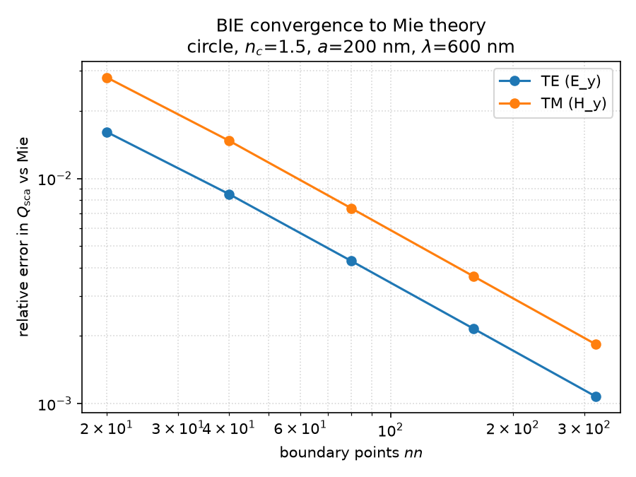
Relative error of the scattering efficiency Q_sca versus the number of
boundary points, converging toward analytic Mie theory (both polarisations):
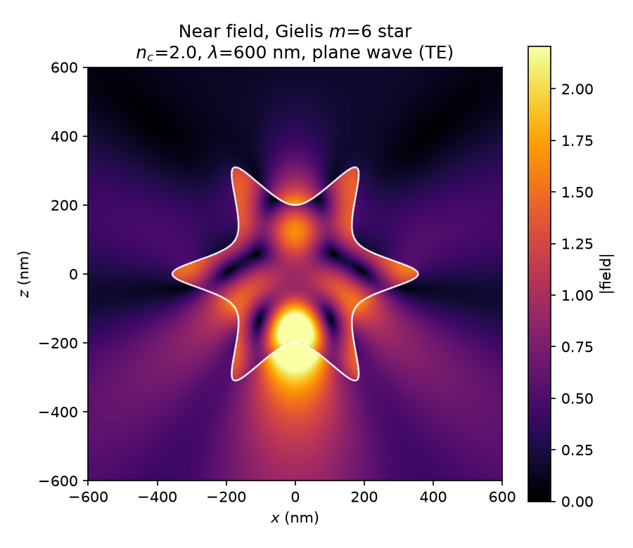
Near field of a Gielis m = 6 star under plane-wave illumination (scattered
field outside the boundary, internal field inside):
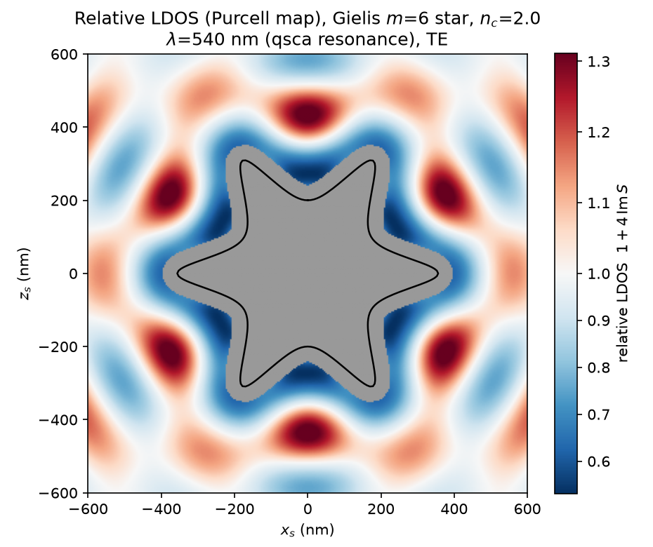
Relative local density of states (Purcell map) around the same Gielis m = 6
star, at one of its qsca resonances: a line-dipole emitter placed in a red
lobe decays faster than in free space (1 + 4·Im S > 1), while blue regions
suppress it. The six-fold pattern mirrors the particle's symmetry. The drive
and the decay rate of an embedded emitter both come from this map — it is the
entry point of quantum-dynamics calculations downstream:
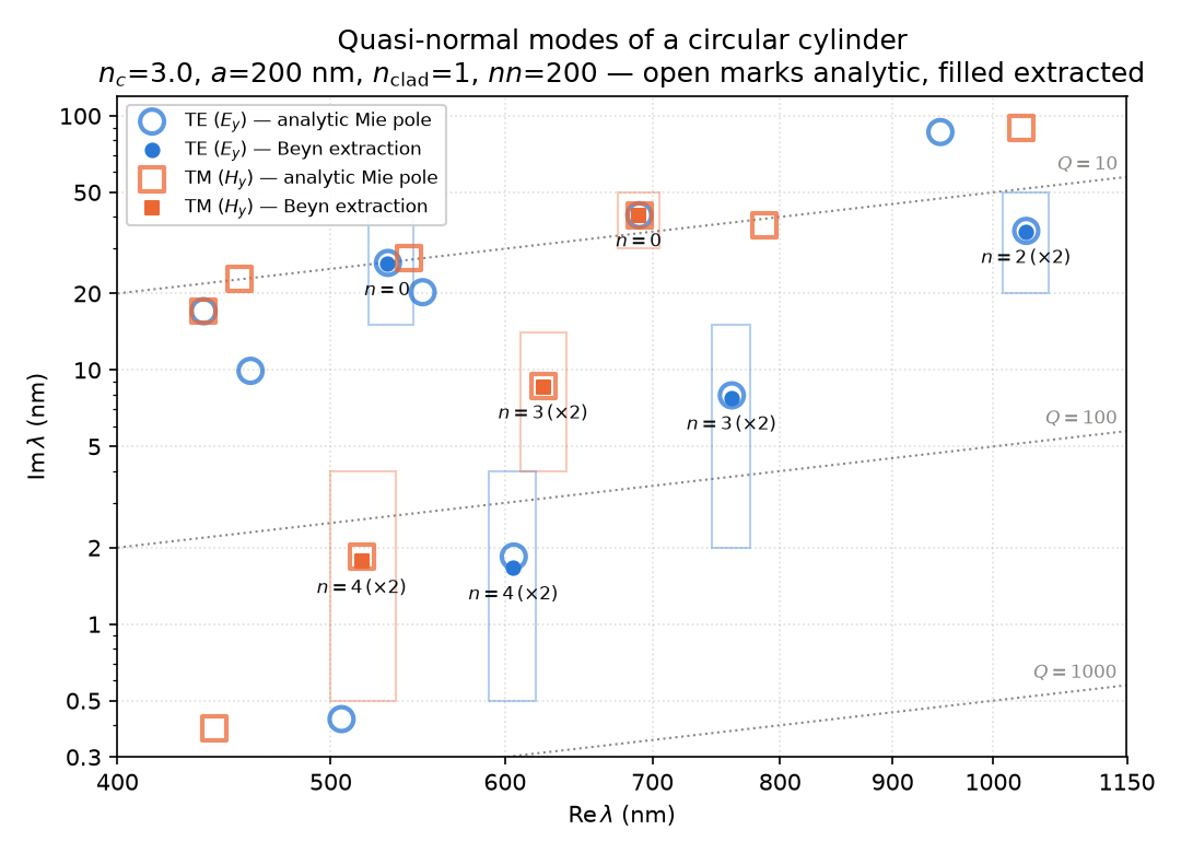
Quasi-normal modes of a circular cylinder in the complex wavelength plane,
extracted from seven search boxes and plotted over the analytic Mie poles of the
same cylinder (open marks analytic, filled extracted). The axes are log-log so
that each iso-Q contour is a straight line, since Q = Re λ / (2 Im λ):
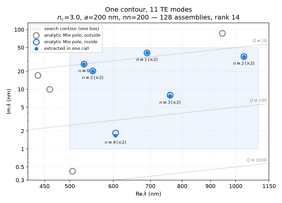
The same physics, one contour. A single rectangle spanning 600 nm of Re λ
returns all eleven TE modes inside it — counting the doubly degenerate pairs
— from one call and 128 matrix assemblies. Beyn's method costs
4·n_quad_per_side assemblies whatever is inside the contour, so eleven modes
cost no more than one; only the probe count has to exceed the mode count. Grey
marks are poles outside the box (three of them leak a rank direction in, hence
rank = 14 against 11 modes):
Regenerate them with:
uv run python examples/convergence_study.py
uv run python examples/nearfield_map.py
uv run python examples/purcell_map.py
uv run python examples/qnm_spectrum.py
uv run python examples/qnm_wide_window.py
Formulation (summary)
- The cylinder is invariant along its axis, so Maxwell reduces to a scalar
Helmholtz problem for one field component (
E_yfor TE,H_yfor TM). - The self-consistent field solution is given everywhere in terms of the surface field and its normal derivative; matching across the interface gives a Fredholm integral equation of the second kind.
- Discretising the boundary with
nnquadrature points yields a dense2nn × 2nncomplex systemM(λ)·ei = rhs, solved directly. - The logarithmic Green-function singularity is handled analytically in the diagonal terms; complex wavenumbers are supported throughout.
- Lengths are in nm, the time convention is
exp(-iωt), and outgoing waves areH_n^{(1)}. - Wavelengths are vacuum wavelengths.
Material.n_core,Material.n_cladandMaterial.epsiare absolute; the background index enters through the single conversionMaterial.wnum_bg(λ_vac) = 2π·n_clad/λ_vac, and the operator sees only background-relative quantities (Material.nc,Material.eps). The Mie size parameterx = 2π·n_clad·rad/λ_vacis exposed as the derivedpysie2d.size_parameter(circular geometry only).
Full details and every sign/layout convention are in docs/conventions.md. The analytic reference is Bohren & Huffman, Absorption and Scattering of Light by Small Particles, ch. 8; the boundary-integral approach follows Maradudin, Michel, McGurn & Méndez, Enhanced backscattering of light from a random grating, Ann. Phys. 203 (1990) 255–307, developed there for randomly rough surfaces; this implementation uses the closed-surface (particle) form given in Valencia et al..
Validation
The physics test suite compares the solver against analytic Mie theory for a
circular cylinder: scattering / extinction / absorption efficiencies, the
optical theorem on a lossy particle, energy conservation on a lossless one, the
convergence rate, and the 2-D 1/√(kr) far-field decay. At nn = 300 the
efficiencies agree with Mie to a few parts in 10³; the error decreases with
nn until it reaches the fixed angular-quadrature floor of the far-field
integrator. See tests/ for the exact tolerances and the reasoning behind them.
The line-dipole / self-Green machinery (v0.2) is validated the same way:
reciprocity of the scattered field (to 10⁻⁶), the free-space limit
(LDOS → 1 far from the particle), LDOS positivity, and — the strong anchor —
the self-Green function of a circular cylinder against its closed-form
Graf-addition-theorem sum on both Re S and Im S. That near-field anchor
converges at first order in nn, so it is run at nn = 1000 to reach 1 %;
the resolved scattered-field sign convention is recorded in
docs/conventions.md.
Quasi-normal-mode extraction (v0.4) is anchored the same way, in three
independent layers: the analytic Mie poles are located first and their
completeness checked against a winding-number count; the contour algorithm is
checked on synthetic matrix pencils with known spectra; and only then is the
composition tested — that the BIE operator's singularities are the Mie poles,
to within its discretisation error and nothing more. That error converges at
first order in nn, in both Re λ and Im λ.
Install / run / test
Requires Python 3.12 and uv.
uv sync                       # create the environment
uv run pytest                 # run the validation suite
uv run ruff format --check .  # formatting
uv run ruff check .           # lint
Minimal use:
from pysie2d import BIESolver, Geometry, Material

geom = Geometry.gielis(rad=200, n_pts=300, m=0)   # circular cylinder, nm
mat = Material(n_core=1.5, n_clad=1.0, pol=2)      # TE
result = BIESolver(geom, mat).scatter(wavelength=600.0)  # vacuum nm

print(result.efficiencies())                       # {'qsca', 'qext', 'qabs'}
Line-dipole emitter and Purcell effect:
from pysie2d import BIESolver, Geometry, Material, relative_ldos

geom = Geometry.gielis(rad=200, n_pts=300, m=6, n1=6, n2=12, n3=12)  # Gielis star
solver = BIESolver(geom, Material(n_core=2.0))
# wavelength is vacuum nm; the LDOS is relative to the unbounded background
print(relative_ldos(solver, wavelength=540.0, x_s=430.0, z_s=0.0))
Quasi-normal modes
A quasi-normal mode is a source-free solution: a complex wavelength where the
boundary-integral operator M(λ) is singular. QNMSolver finds every mode
inside a rectangle of the complex λ-plane by contour integration (Beyn's
method) — no initial guess and no scan, at a cost independent of how many modes
are inside.
from pysie2d import Geometry, Material, QNMSolver

geom = Geometry.gielis(rad=200, n_pts=200, m=0)
mat = Material(n_core=3.0, n_clad=1.0, pol=2)             # TE
res = QNMSolver(geom, mat).modes(745 + 2j, 775 + 15j)     # box corners, vacuum nm

print(res.wavelengths)      # 760.326 + 7.770j, twice — a degenerate pair
print(res.quality_factors)  # Q = Re λ / (2 Im λ)
print(res.edge_margin)      # contour-quality diagnostic; near zero is a warning
Search boxes must lie in Im λ > 0 (the decaying half-plane under exp(-iωt))
and Re λ > 0 (which keeps M(λ) holomorphic); both are asserted. Poles do
not come in conjugate pairs here, and every n ≥ 1 mode of a circle is
doubly degenerate.
Read docs/qnm-guide.md
before using this — it covers how to place a box, how to read the diagnostics,
what refine() does and does not buy you, and the limitations the feature ships
with.
Mode sensitivity
QNMResult.sensitivity(at) returns dλ/dp for every mode from the adjoint
quotient − uᴴ(∂M/∂p)v / uᴴ(∂M/∂λ)v, re-extracting no eigenvalue. at is a
callable δ → (geometry, material), so a shape parameter and a refractive index
go through one signature and one code path.
res = QNMSolver(geom, mat).modes(745 + 2j, 775 + 15j).refine()
theta = res.geometry.theta                     # the node set must be frozen

def wider(delta):                              # dλ/db, b in its own units
    return Geometry.gielis(rad=200, n_pts=200, theta=theta,
                           m=4, b=1.2 + delta), mat

print(res.sensitivity(wider))
The geometry at returns must carry res.geometry.theta exactly — a shape
derivative holds the node set fixed, and differentiating the arc-length
parametrisation along with the physics costs two orders of convergence. Degenerate
poles dispatch to a secular problem rather than raising. dλ/dp converges at
first order in n_pts, so richardson_limit extrapolates two rungs to the limit
for less than the cost of one finer one. Conventions
§10,
§11 and §12 carry the details and the measured anchors.
Performance
The system is a dense 2nn × 2nn complex matrix; at nn = 300 (a 600 × 600
solve) a single wavelength takes below one second in a modern computer, so wavelength
sweeps are cheap serial for loops — no parallelism required.
Matrix assembly dominates a single solve, and almost all of that cost is Hankel
evaluation. For real arguments H_n^{(1)} = J_n + i·Y_n exactly, and the Cephes
J_n/Y_n kernels are an order of magnitude faster than the general
complex-argument algorithm — so hank0/hank1/cbesh dispatch on the argument
at runtime, making assemble_matrix about 5× faster for a non-absorbing
particle and 1.8× for an absorbing one. Complex wavenumbers take the original
path and are bit-identical, which is what keeps quasi-normal-mode work possible.
For a Purcell map, every grid point is a different source position, hence a
different right-hand side — but the matrix M(λ) is the same for all of them.
relative_ldos_map therefore factorises M once with
scipy.linalg.lu_factor and reuses it across all sources, and it batches the
reuse: one multi-RHS BLAS-3 lu_solve and one vectorised representation-formula
evaluation per chunk rather than a per-point loop (7.5× per source point). What
would be an hour-long sweep takes seconds.
Roadmap
- v0.1.0 — core scattering: plane-wave excitation, near/far fields, cross-section efficiencies, Mie validation, convergence study, CI.
- v0.2.0 — line-dipole (point-source) excitation and the self-Green function → relative LDOS / Purcell maps.
- v0.3.0 — performance: Cephes fast path for real-argument Hankel
functions and a batched, factorise-once
relative_ldos_map. - v0.4.0 — vacuum-wavelength and background-index conventions (breaking), and quasi-normal-mode extraction via Beyn's contour method, validated against analytic Mie resonances.
- v0.4.2 — exact scale covariance of the discrete BIE system, recorded as conventions §9.
- v0.5.0 — threaded contour integration in
contour_moments, and an adjoint eigenvalue-sensitivity API (dλ/dpper mode) on top of the identity already proved in conventions §9. (latest release) No breaking changes; every v0.4.x call still means what it meant.
What v0.5 adds to Geometry
Geometry now records the boundary node angles it was built on, as
Geometry.theta, and Geometry.gielis accepts theta= to build a shape on
angles supplied from elsewhere:
base  = Geometry.gielis(rad=200, n_pts=200, m=4, b=1.2)   # unchanged
wider = Geometry.gielis(rad=200, n_pts=200, m=4, b=1.3,
                        theta=base.theta)                 # new: same node set
Both arguments are optional and both are additions — Geometry.gielis places
nodes by uniform arc length when you omit theta, exactly as before, and
Geometry(...) built directly from your own arrays works without one, leaving
theta as None. Scattering, fields, LDOS and mode extraction never read it.
It exists for shape derivatives. QNMResult.sensitivity evaluates M(p₀−h) and
M(p₀+h) and must do so on the same node set; if the nodes are re-placed
between the two, the difference quotient differentiates the arc-length
parametrisation along with the physics. That error term is O(h) rather than
O(h²), it is not monotone in h, and it grows with n_pts — the one error
in this package that refinement makes worse. Freezing the nodes takes the
measured convergence rate on ∂M/∂b from 2.7 to 100.1, against an ideal of 100.
So sensitivity refuses a geometry with no node set, and names which one is
missing, rather than falling back to re-inversion — a fallback would return a
wrong answer that looks exactly like a right one. Conventions
§10.
License
MIT — see LICENSE.
1 maintainer

Download files
Download the file for your platform. If you're not sure which to choose, learn more about installing packages.
Source Distribution
Built Distribution
Filter files by name, interpreter, ABI, and platform.
If you're not sure about the file name format, learn more about wheel file names.
Copy a direct link to the current filters
File details
Details for the file pysie2d-0.5.0.tar.gz.
File metadata
- Download URL: pysie2d-0.5.0.tar.gz
- Upload date:
- Size: 57.9 kB
- Tags: Source
- Uploaded using Trusted Publishing? Yes
- Uploaded via:
uv/0.12.9 {"installer":{"name":"uv","version":"0.12.9","subcommand":["publish"]},"python":null,"implementation":{"name":null,"version":null},"distro":{"name":"Ubuntu","version":"24.04","id":"noble","libc":null},"system":{"name":null,"release":null},"cpu":null,"openssl_version":null,"setuptools_version":null,"rustc_version":null,"ci":true}
File hashes
| Algorithm | Hash digest | |
|---|---|---|
| SHA256 |
67e0dc57bc26c8098664c00cec93e9c2314dc88524e725b4b2df6535d9c938c7
|
|
| MD5 |
ab25e5ed65ae5984e2b1806bd6cb20b3
|
|
| BLAKE2b-256 |
db5f2a3b0217c7510189673d3a6945742359e1b232df79d330debd6917fe6163
|
File details
Details for the file pysie2d-0.5.0-py3-none-any.whl.
File metadata
- Download URL: pysie2d-0.5.0-py3-none-any.whl
- Upload date:
- Size: 64.1 kB
- Tags: Python 3
- Uploaded using Trusted Publishing? Yes
- Uploaded via:
uv/0.12.9 {"installer":{"name":"uv","version":"0.12.9","subcommand":["publish"]},"python":null,"implementation":{"name":null,"version":null},"distro":{"name":"Ubuntu","version":"24.04","id":"noble","libc":null},"system":{"name":null,"release":null},"cpu":null,"openssl_version":null,"setuptools_version":null,"rustc_version":null,"ci":true}
File hashes
| Algorithm | Hash digest | |
|---|---|---|
| SHA256 |
28968ff8d28d535cc8276e5d286042920ac514edb79636b827959ba6dc7c1e50
|
|
| MD5 |
9ec519aaebb7376e2bf26f0e2ad65fdc
|
|
| BLAKE2b-256 |
0fc35aaf4b1f997730b9233353b012a4c54b3af8af3087243656b0c585f69e47
|














