A python package designed to work with spectroscopy data

Project description
Pyspectra
Welcome to pyspectra.
This package is intended to put functions together to analyze and transform spectral data from multiple spectroscopy instruments.
Currently supported input files are:
- .spc
- .dx
PySpectra is intended to facilitate working with spectroscopy files in python by using a friendly integration with pandas dataframe objects.
.
Also pyspectra provides a set of routines to execute spectral pre-processing like:
- MSC
- SNV
- Detrend
- Savitzky - Golay
- Derivatives
- ..
Data spectra can be used for traditional chemometrics analysis but also can be used in general advanced analytics modelling in order to deliver additional information to manufacturing models by supplying spectral information.
#Import basic libraries
import spc
import matplotlib.pyplot as plt
import numpy as np
import pandas as pd
from sklearn.decomposition import PCA
Read .spc file
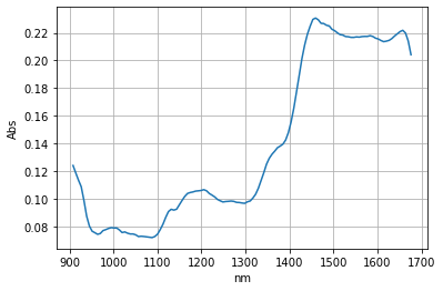
Read a single file
from pyspectra.readers.read_spc import read_spc
spc=read_spc('pyspectra/sample_spectra/VIAVI/JDSU_Phar_Rotate_S06_1_20171009_1540.spc')
spc.plot()
plt.xlabel("nm")
plt.ylabel("Abs")
plt.grid(True)
print(spc.head())
gx-y(1)
908.100000    0.123968
914.294355    0.118613
920.488710    0.113342
926.683065    0.108641
932.877419    0.098678
dtype: float64
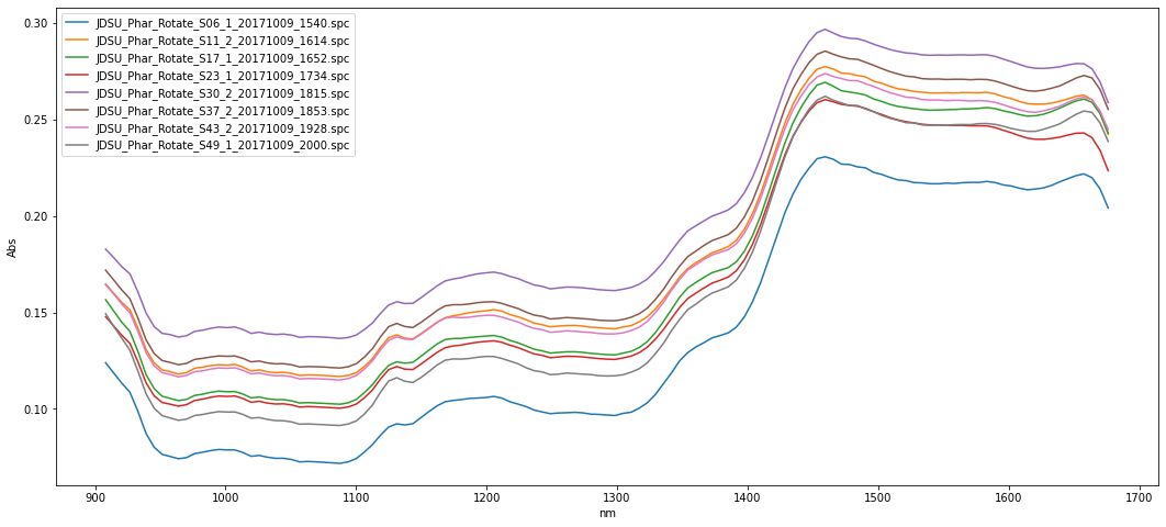
Read multiple .spc files from a directory
from pyspectra.readers.read_spc import read_spc_dir

df_spc, dict_spc=read_spc_dir('pyspectra/sample_spectra/VIAVI')
display(df_spc.transpose())
f, ax =plt.subplots(1, figsize=(18,8))
ax.plot(df_spc.transpose())
plt.xlabel("nm")
plt.ylabel("Abs")
ax.legend(labels= list(df_spc.transpose().columns))
plt.show()
gx-y(1)
gx-y(1)
gx-y(1)
gx-y(1)
gx-y(1)
gx-y(1)
gx-y(1)
gx-y(1)
.dataframe tbody tr th {
    vertical-align: top;
}

.dataframe thead th {
    text-align: right;
}
| JDSU_Phar_Rotate_S06_1_20171009_1540.spc | JDSU_Phar_Rotate_S11_2_20171009_1614.spc | JDSU_Phar_Rotate_S17_1_20171009_1652.spc | JDSU_Phar_Rotate_S23_1_20171009_1734.spc | JDSU_Phar_Rotate_S30_2_20171009_1815.spc | JDSU_Phar_Rotate_S37_2_20171009_1853.spc | JDSU_Phar_Rotate_S43_2_20171009_1928.spc | JDSU_Phar_Rotate_S49_1_20171009_2000.spc | |
|---|---|---|---|---|---|---|---|---|
| 908.100000 | 0.123968 | 0.164750 | 0.156647 | 0.147828 | 0.182833 | 0.171957 | 0.164471 | 0.149373 |
| 914.294355 | 0.118613 | 0.159980 | 0.150746 | 0.142974 | 0.178452 | 0.166827 | 0.159545 | 0.142818 |
| 920.488710 | 0.113342 | 0.155193 | 0.144959 | 0.138178 | 0.173734 | 0.161695 | 0.154330 | 0.136648 |
| 926.683065 | 0.108641 | 0.151398 | 0.140178 | 0.134014 | 0.170061 | 0.157110 | 0.149876 | 0.130452 |
| 932.877419 | 0.098678 | 0.141859 | 0.129715 | 0.124426 | 0.160590 | 0.147076 | 0.140119 | 0.119561 |
| ... | ... | ... | ... | ... | ... | ... | ... | ... |
| 1651.422581 | 0.220935 | 0.262070 | 0.259643 | 0.242916 | 0.279041 | 0.271492 | 0.260664 | 0.252704 |
| 1657.616935 | 0.221848 | 0.262732 | 0.260664 | 0.243092 | 0.278962 | 0.272893 | 0.261647 | 0.254481 |
| 1663.811290 | 0.219904 | 0.260335 | 0.258975 | 0.240656 | 0.276382 | 0.271624 | 0.260278 | 0.253761 |
| 1670.005645 | 0.214080 | 0.253475 | 0.253110 | 0.234047 | 0.269528 | 0.265615 | 0.254568 | 0.248288 |
| 1676.200000 | 0.204217 | 0.242375 | 0.243082 | 0.223539 | 0.258771 | 0.255306 | 0.244826 | 0.238663 |
125 rows × 8 columns
Read .dx spectral files
Pyspectra is also built with a set of regex that allows to read the most common .dx file formats from different vendors like:
- FOSS
- Si-Ware Systems
- Spectral Engines
- Texas Instruments
- VIAVI
Read a single .dx file
.dx reader can read:
- Single files containing single spectra : read
- Single files containing multiple spectra : read
- Multiple files from directory : read_from_dir
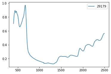
Single file, single spectra
# Single file with single spectra
from pyspectra.readers.read_dx import read_dx
#Instantiate an object
Foss_single= read_dx()
# Run  read method
df=Foss_single.read(file='pyspectra/sample_spectra/DX multiple files/Example1.dx')
df.transpose().plot()
<matplotlib.axes._subplots.AxesSubplot at 0x1f44faa7940>
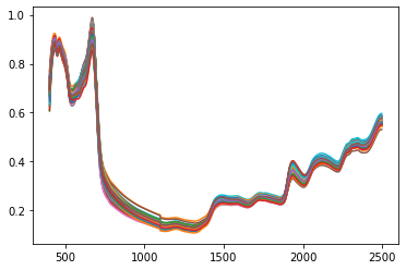
Single file, multiple spectra:
.dx reader stores all the information as attributes of the object on Samples. Each key represent a sample.
Foss_single= read_dx()
# Run  read method
df=Foss_single.read(file='pyspectra/sample_spectra/FOSS/FOSS.dx')
df.transpose().plot(legend=False)
<matplotlib.axes._subplots.AxesSubplot at 0x1f44f7f2e50>
for c in Foss_single.Samples['29179'].keys():
    print(c)
y
Conc
TITLE
JCAMP_DX
DATA TYPE
CLASS
DATE
DATA PROCESSING
XUNITS
YUNITS
XFACTOR
YFACTOR
FIRSTX
LASTX
MINY
MAXY
NPOINTS
FIRSTY
CONCENTRATIONS
XYDATA
X
Y
Spectra preprocessing
Pyspectra has a set of built in classes to perform spectra pre-processing like:
- MSC: Multiplicative scattering correction
- SNV: Standard normal variate
- Detrend
- n order derivative
- Savitzky golay smmothing
from pyspectra.transformers.spectral_correction import msc, detrend ,sav_gol,snv
MSC= msc()
MSC.fit(df)
df_msc=MSC.transform(df)


f, ax= plt.subplots(2,1,figsize=(14,8))
ax[0].plot(df.transpose())
ax[0].set_title("Raw spectra")

ax[1].plot(df_msc.transpose())
ax[1].set_title("MSC spectra")
plt.show()

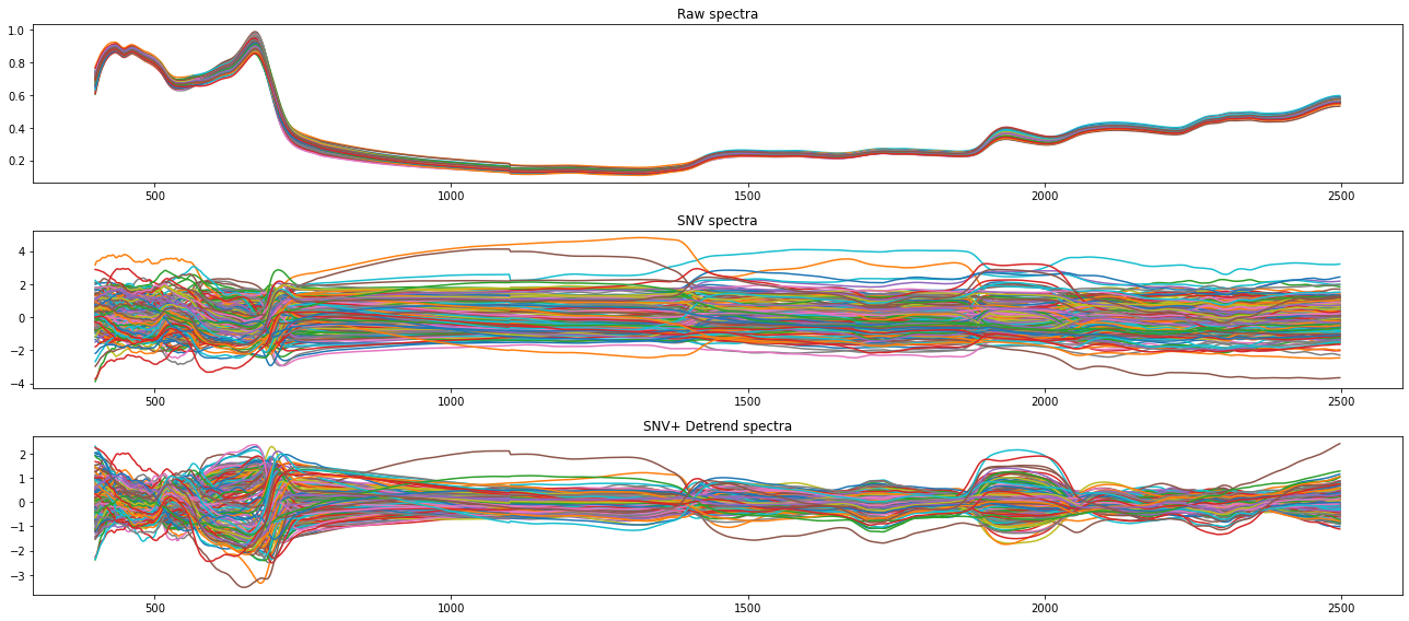
SNV= snv()
df_snv=SNV.fit_transform(df)

Detr= detrend()
df_detrend=Detr.fit_transform(spc=df_snv,wave=np.array(df_snv.columns))

f, ax= plt.subplots(3,1,figsize=(18,8))
ax[0].plot(df.transpose())
ax[0].set_title("Raw spectra")

ax[1].plot(df_snv.transpose())
ax[1].set_title("SNV spectra")

ax[2].plot(df_detrend.transpose())
ax[2].set_title("SNV+ Detrend spectra")

plt.tight_layout()
plt.show()
Modelling of spectra
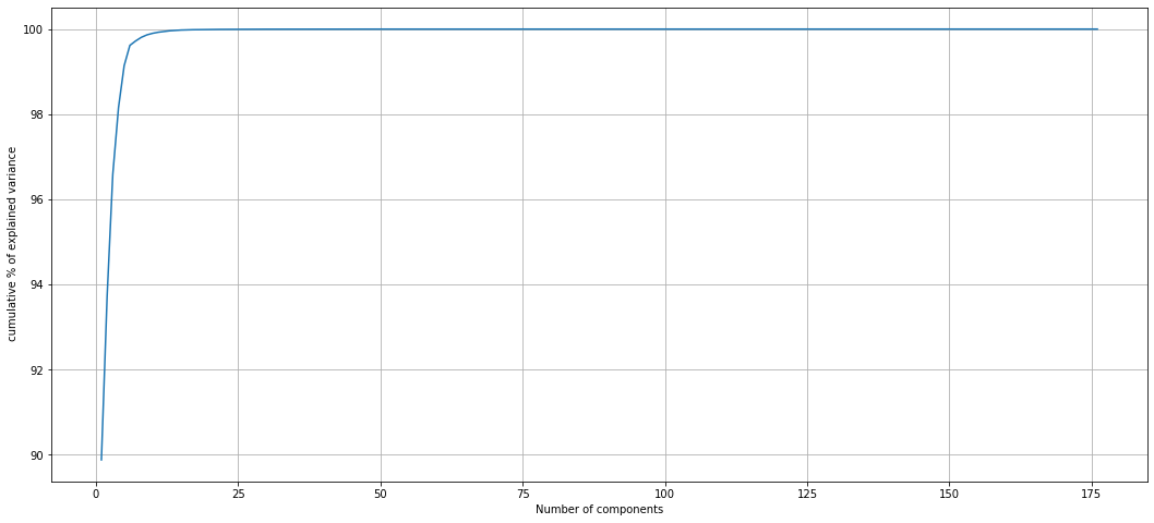
Decompose using PCA
pca=PCA()
pca.fit(df_msc)
plt.figure(figsize=(18,8))
plt.plot(range(1,len(pca.explained_variance_)+1),100*pca.explained_variance_.cumsum()/pca.explained_variance_.sum())
plt.grid(True)
plt.xlabel("Number of components")
plt.ylabel(" cumulative % of explained variance")
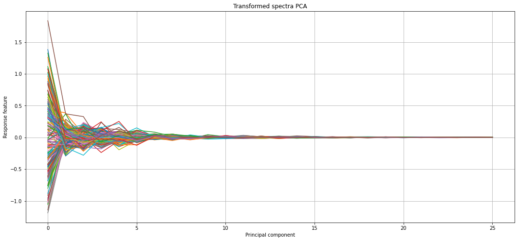
df_pca=pd.DataFrame(pca.transform(df_msc))
plt.figure(figsize=(18,8))
plt.plot(df_pca.loc[:,0:25].transpose())


plt.title("Transformed spectra PCA")
plt.ylabel("Response feature")
plt.xlabel("Principal component")
plt.grid(True)
plt.show()
Using automl libraries to deploy faster models
import tpot
from tpot import TPOTRegressor
from sklearn.model_selection import RepeatedKFold
cv = RepeatedKFold(n_splits=10, n_repeats=3, random_state=1)
model = TPOTRegressor(generations=10, population_size=50, scoring='neg_mean_absolute_error',
                      cv=cv, verbosity=2, random_state=1, n_jobs=-1)
y=Foss_single.Conc[:,0]
x=df_pca.loc[:,0:25]
model.fit(x,y)
HBox(children=(FloatProgress(value=0.0, description='Optimization Progress', max=550.0, style=ProgressStyle(de…


Generation 1 - Current best internal CV score: -0.30965836730187607

Generation 2 - Current best internal CV score: -0.30965836730187607

Generation 3 - Current best internal CV score: -0.30965836730187607

Generation 4 - Current best internal CV score: -0.308295313408046

Generation 5 - Current best internal CV score: -0.308295313408046

Generation 6 - Current best internal CV score: -0.308295313408046

Generation 7 - Current best internal CV score: -0.308295313408046

Generation 8 - Current best internal CV score: -0.3082953134080456

Generation 9 - Current best internal CV score: -0.3082953134080456

Generation 10 - Current best internal CV score: -0.3078569602146527

Best pipeline: LassoLarsCV(PCA(LinearSVR(input_matrix, C=0.1, dual=True, epsilon=0.1, loss=epsilon_insensitive, tol=0.01), iterated_power=3, svd_solver=randomized), normalize=False)


TPOTRegressor(cv=RepeatedKFold(n_repeats=3, n_splits=10, random_state=1),
              generations=10, n_jobs=-1, population_size=50, random_state=1,
              scoring='neg_mean_absolute_error', verbosity=2)
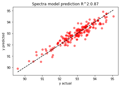
from sklearn.metrics import r2_score
r2=round(r2_score(y,model.predict(x)),2)
plt.scatter(y,model.predict(x),alpha=0.5, color='r')
plt.plot([y.min(),y.max()],[y.min(),y.max()],LineStyle='--',color='black')
plt.xlabel("y actual")
plt.ylabel("y predicted")
plt.title("Spectra model prediction R^2:"+ str(r2))

plt.show()
Release history Release notifications | RSS feed


Download files
Download the file for your platform. If you're not sure which to choose, learn more about installing packages.
Source Distribution
Built Distribution
Filter files by name, interpreter, ABI, and platform.
If you're not sure about the file name format, learn more about wheel file names.
Copy a direct link to the current filters
File details
Details for the file pyspectra-0.0.1.2.tar.gz.
File metadata
- Download URL: pyspectra-0.0.1.2.tar.gz
- Upload date:
- Size: 14.2 kB
- Tags: Source
- Uploaded using Trusted Publishing? No
- Uploaded via: twine/3.2.0 pkginfo/1.6.1 requests/2.24.0 setuptools/47.1.0 requests-toolbelt/0.9.1 tqdm/4.51.0 CPython/3.8.5
File hashes
| Algorithm | Hash digest | |
|---|---|---|
| SHA256 |
2b31be5a7a31883f105ea286fa272fe1b1e70ce551ae34d11028267392df04e6
|
|
| MD5 |
9e042b1ea94f8fd9b09283071701f92d
|
|
| BLAKE2b-256 |
d2db5596a5300bcfd5844138b9097c01b6672680005c5a98b97881c43400b57e
|
File details
Details for the file pyspectra-0.0.1.2-py3-none-any.whl.
File metadata
- Download URL: pyspectra-0.0.1.2-py3-none-any.whl
- Upload date:
- Size: 22.6 kB
- Tags: Python 3
- Uploaded using Trusted Publishing? No
- Uploaded via: twine/3.2.0 pkginfo/1.6.1 requests/2.24.0 setuptools/47.1.0 requests-toolbelt/0.9.1 tqdm/4.51.0 CPython/3.8.5
File hashes
| Algorithm | Hash digest | |
|---|---|---|
| SHA256 |
ad0965ee554f0fb4d2e2982d95f7c315195206faba30960200956d213f49f154
|
|
| MD5 |
463336238d2c8d835b2bc5430824b298
|
|
| BLAKE2b-256 |
34cd072c984e3a3130f1f1dd9423c8e1a97b312cb09f616ebcd8ba09b9b0f03d
|


