


ToMATo
ToMATo (Topological Mode Analysis Tool) quickly finds intuitive clusters in data by choosing the most topologically persistent modes of a density estimate (or any other vertex function) on a neighborhood graph.
Author: Kenneth Howe
Installation
pip install pytomato
Note: the package is installed as pytomato but imported as tomato.
Quick Start
The ToMATo class conforms to the sklearn API.
from tomato import ToMATo
from sklearn.datasets import make_blobs

X, _ = make_blobs(1_000, random_state=42)

clf = ToMATo()
labels = clf.fit_predict(X)

ToMATo Example Clustering.
How It Works
ToMATo chooses the most topologically persistent clusters in a neighborhood graph with respect to a vertex function, typically a smooth density estimate. Its clusters therefore correspond to persistent modes of that function, rather than to components of an arbitrary distance or density threshold.
Intuitively, each cluster is a peak of the vertex function. A peak's persistence is how far it rises above the level where it merges into a taller peak, so low-persistence peaks are treated as noise in the function rather than as real clusters. For readers unfamiliar with topological persistence, this blog post by Christian Bock provides a concise introduction.
ToMATo was originally introduced as an algorithm for finding clusters in any graph equipped with any vertex function. This repository preserves that generic form via the ToMAToCore class, which takes a graph and vertex function directly. For general-purpose clustering of point cloud data, ToMATo fixes the choice of graph and vertex function, using the RMS distance estimator of distance to a measure (Chazal et al., 2011) on a KNN graph, as used in the original paper. This addresses the needs of the most common spatial clustering use cases; however, the underlying algorithm is a highly extensible, general framework for graph clustering, with applications extending to network analysis, geographic regionalization, and other graph-based modeling tasks.
The theory behind ToMATo provides a concise framework for a number of features valuable to a clustering tool:
- Fast, hierarchical, density-based clustering
- Optional noise-awareness
- Optional number of clusters specification
- Assignment probabilities and soft clustering
- Out-of-sample prediction
- Spatially constrained regionalization
Features
Persistence threshold selection
Several methods are available for selecting the persistence threshold:
- Profile-likelihood split (default).
- This method attempts to automatically find a threshold which separates significant clusters from noisy ones by finding a "big gap" or "elbow" in the persistence diagram.
- Maximum persistence gap.
- This method is best for choosing only the most stable, high-confidence clusters.
- User-specified persistence threshold.
- Exposed for advanced users who may want to design their own criteria for selecting persistence thresholds.
- A threshold chosen for a specified number of clusters.
- See next section.
# Default: Automatic profile-likelihood selection
clf = ToMATo().fit(X)

# Optional: Largest persistence gap selection
clf = ToMATo(cluster_selection_method="max_jump").fit(X)

# Optional: Explicit persistence threshold
threshold_clf = ToMATo(persistence_threshold=0.2).fit(X)
Number of clusters specification
Because the spanning tree can be cut at a depth that guarantees an exact number of surviving nodes, ToMATo can return a fixed number of clusters when required. Alternatively, a minimum number of clusters can be specified, for example to prevent ToMATo from returning a single cluster.
# Fixed number clusters
clf = ToMATo(n_clusters=3).fit(X)

# Minimum number of clusters
clf = ToMATo(min_clusters=3).fit(X)
Noise-aware labeling
ToMATo computes a pointwise assignment strength for a given clustering by comparing each point's local function value to the cluster average. An assignment strength threshold (50% by default) can be specified to classify points as noise when their strength falls below it; such points receive the label -1.
# Run with noise awareness (i.e. return >50% confidence labels)
clf = ToMATo(noise_aware=True).fit(X)
labels = clf.labels_  # Noise labeled -1

# Optional: Specify a custom threshold after fit
clf = ToMATo(...).fit(X)
labels = clf.noise_aware_labels(threshold=0.9)
Soft clustering
Assignment probabilities can also be computed for every cluster in a labeling, enabling soft clustering in near-linear time.
clf = ToMATo(...).fit(X)
probs = clf.full_assignment_probabilities(temperature=1.0)
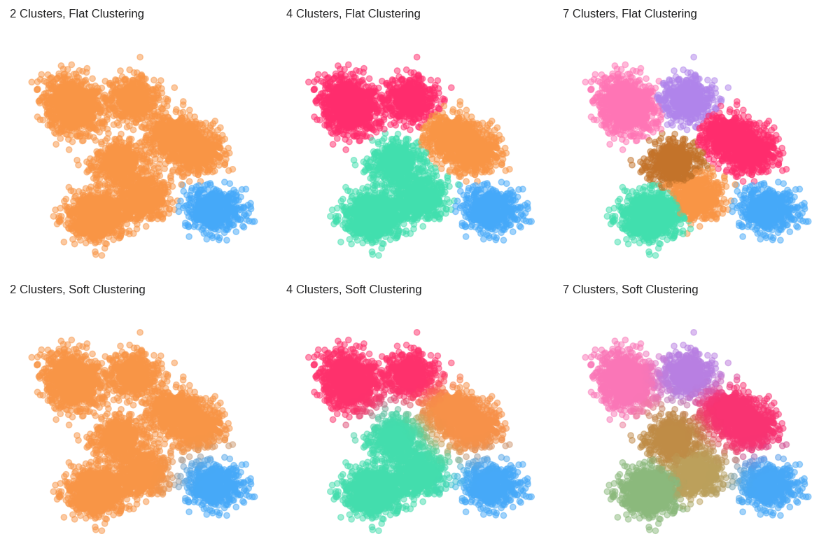
ToMATo Soft Clustering Example with Color Blending.
Out-of-sample prediction
A fitted ToMATo clusterer can assign labels to previously unseen points.
clf = ToMATo().fit(X_train)
labels = clf.predict(X_new)
Advanced Usage
Precomputed graphs and functions with ToMAToCore
The ToMAToCore class exposes a fit method that accepts two inputs: graph (a csr_matrix) and f (an np.ndarray). This interface accommodates users who already have data in graph form, who prefer a custom method of graph construction, or who have a custom descriptor function.
from tomato import ToMAToCore

clf = ToMAToCore()
clf.fit(graph, f)
Persistence diagram inspection
ToMATo calculates the 0th-order persistence of piecewise-linear functions on graphs. The ToMATo.graph_persistence_ attribute stores a GraphPersistence object providing access to the persistence diagram, spanning tree, and other persistence data. This can be used to characterize the cluster function or to determine custom persistence thresholds for labeling.
Geographic (spatially constrained) regionalization
Because the core algorithm can cluster any graph equipped with any vertex function, variants can perform spatially constrained clustering, commonly called "geographic regionalization" in geographic applications. The supplied graph should encode the spatial contiguity structure to preserve in the returned regions, and the passed data should encode attributes to cluster on. The GeoToMATo class implements this. The graph can be any csr_matrix encoding spatial contiguity, such as a contiguity matrix from libpysal or one you build yourself.
from tomato.regionalization import GeoToMATo

clf = GeoToMATo()
clf.fit(graph, X)
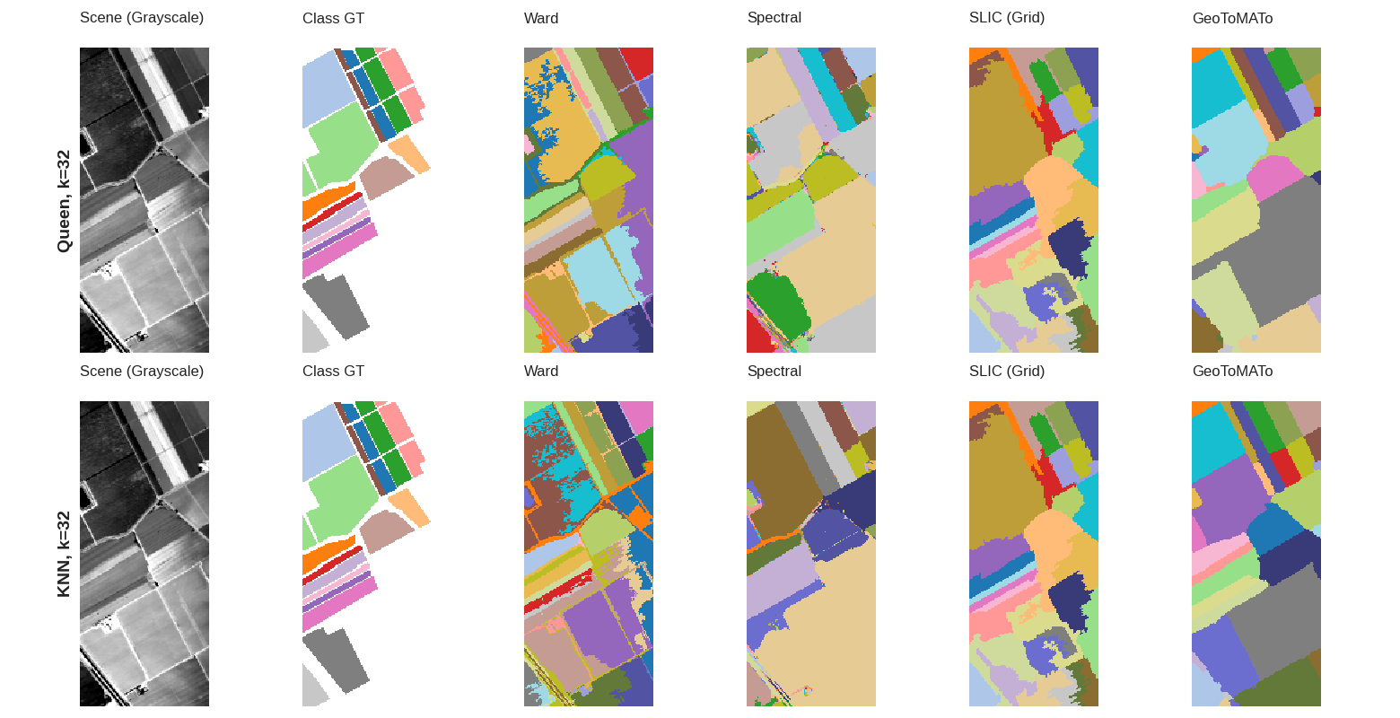
GeoToMATo Regionalization Example on Salinas Valley, CA Hyperspectral Imagery.
Visualization
The ToMAToVisualization class offers methods for visualizing cluster labels, the input graph and vertex function, graph gradients, the merge tree, and the persistence diagram. It is initialized using a fitted instance of the ToMATo clusterer:
from tomato.visualization import ToMAToVisualization

# Assuming `clf` has already been fit on `X`
viz = ToMAToVisualization(clf)
viz.plot_labels(X)
viz.plot_persistence_diagram()
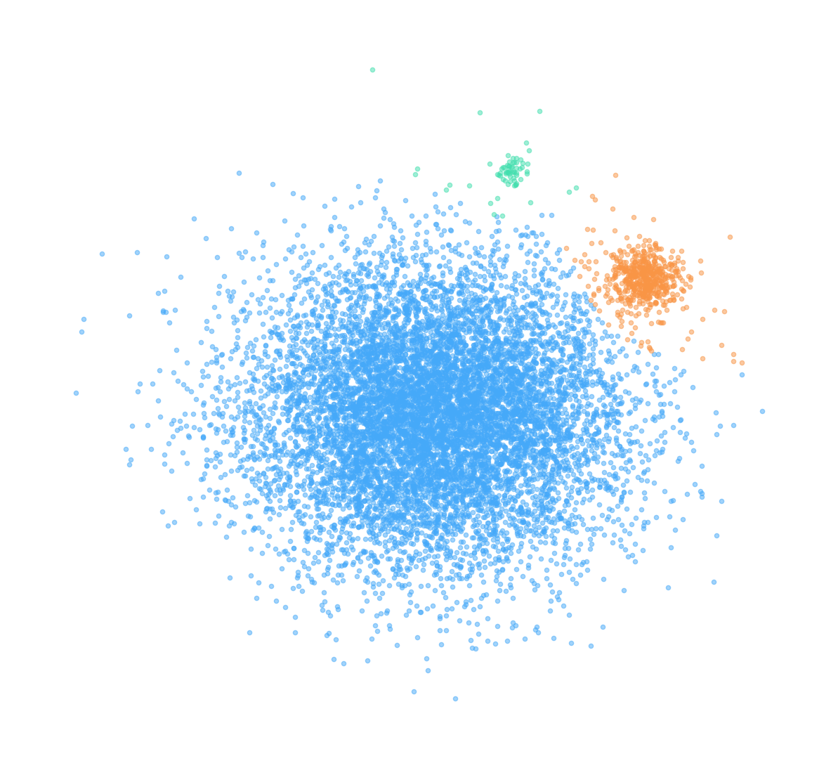
Labels plot.
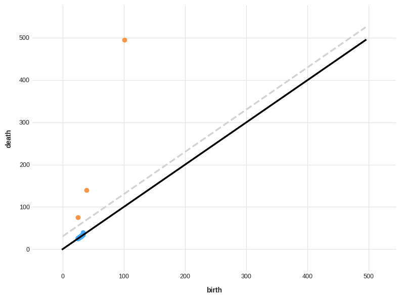
Persistence diagram plot.
Performance
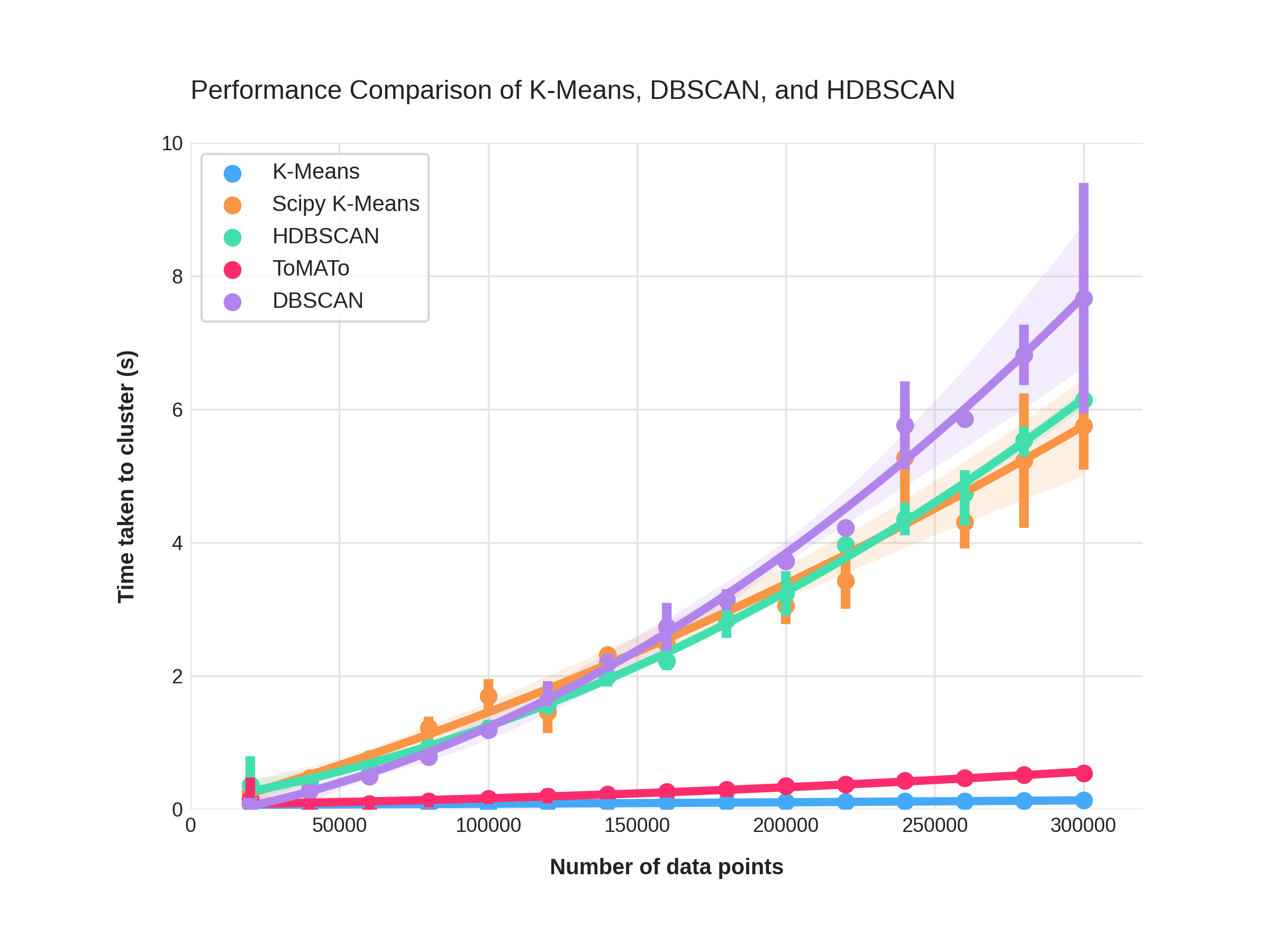
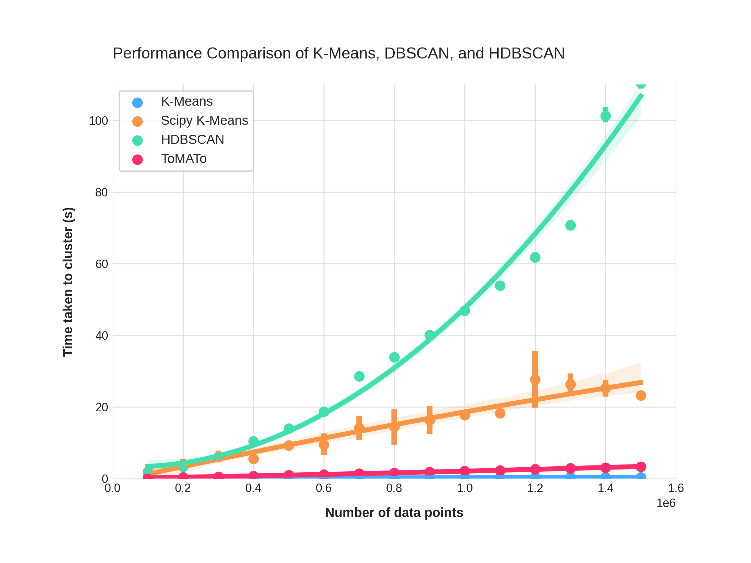
ToMATo runs in near-linear time, making it significantly faster than comparable algorithms such as HDBSCAN, whose complexity is typically worse than $O(n \log n)$.
The following timing results compare ToMATo against DBSCAN, HDBSCAN, and two implementations of K-Means:
Extended to 1.5 million data points, ToMATo maintains near-linear scaling with relatively fast clustering times:
The timing code is included in this repository, adapted from the HDBSCAN repository.
Citation
ToMATo was introduced in 2011 by Chazal, et al.:
Chazal, F., Guibas, L. J., Oudot, S., & Skraba, P. (2011). Persistence-based clustering in Riemannian manifolds. Proceedings of the 27th Annual ACM Symposium on Computational Geometry (SCG '11), 97–106. https://geometry.stanford.edu/paper/cgos-pbcrm-11/cgos-pbcrm-11.pdf
@inproceedings{chazal2011persistence,
  title     = {Persistence-based clustering in Riemannian manifolds},
  author    = {Chazal, Fr{\'e}d{\'e}ric and Guibas, Leonidas J. and Oudot, Steve Y. and Skraba, Primoz},
  booktitle = {Proceedings of the 27th Annual ACM Symposium on Computational Geometry (SCG '11)},
  pages     = {97--106},
  year      = {2011}
}
License
ToMATo is released under the MIT License. See LICENSE for the full license text.
1 maintainer

Metadata
1 maintainer
Release files for pytomato 0.5.1
For a detailed explanation of source distributions (sdists) and built distributions (wheels), please see the package formats documentation.
Source distribution (sdist)
| File | Size | Uploaded | |
|---|---|---|---|
| pytomato-0.5.1.tar.gz | 47.2 kB | Details |
Built distribution (wheel)
| File | Interpreter | ABI | Platform | Reset |
|---|---|---|---|---|
| pytomato-0.5.1-py3-none-any.whl | Python 3 | none | any | Details |
Total release size: 97.2 kB
Release files / pytomato-0.5.1.tar.gz
| Download URL | pytomato-0.5.1.tar.gz |
|---|---|
| Size | 47.2 kB |
| Tags | Source |
|
SHA-256 checksum How to use checksums |
8601c2d96a7cbf695edc0d2cdf3a3af73cee3ef20125aa7efb0b3a33218f9ddb
|
|
BLAKE2b-256 checksum How to use checksums |
2daede5eb5753438b82be249195f8242c8239493b4b0038cd00eb1caafe61dd4
|
| Upload date | |
|
Uploaded using Trusted Publishing? What is trusted publishing? |
No |
| Uploaded via |
twine/7.0.0 CPython/3.11.3
|
Release files / pytomato-0.5.1-py3-none-any.whl
| Download URL | pytomato-0.5.1-py3-none-any.whl |
|---|---|
| Size | 50.0 kB |
| Tags | Python 3 |
|
SHA-256 checksum How to use checksums |
bddf1c8f6cddf6afd550f103289ecdda4f84aa21d997d1dd9f550ccd3b4ff46d
|
|
BLAKE2b-256 checksum How to use checksums |
13e419d70eff5c96fe91c148c0abbc6127b9ba2a965fe163e7b1a97ecf699aa0
|
| Upload date | |
|
Uploaded using Trusted Publishing? What is trusted publishing? |
No |
| Uploaded via |
twine/7.0.0 CPython/3.11.3
|














