PyTorch implementation of Bézier simplex fitting

Project description
PyTorch-BSF


Fit smooth, high-dimensional manifolds to your data — from a single GPU to a multi-node cluster.
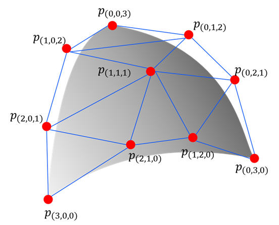
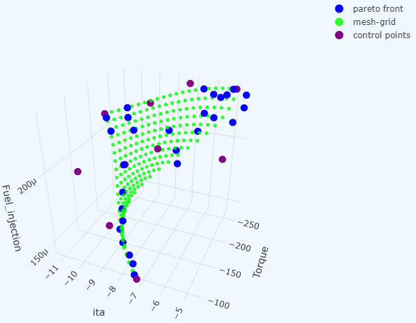
pytorch-bsf brings Bézier simplex fitting to PyTorch. A Bézier simplex is a high-dimensional generalization of the Bézier curve: where a curve models a 1-D path, a Bézier simplex can model an arbitrarily complex point cloud as a smooth parametric hyper-surface in any number of dimensions. This makes it a natural tool for representing Pareto fronts in multi-objective optimization, interpolating scattered observations, and fitting geometric structures in high-dimensional spaces.
Key features:
- Simple, Pythonic API — train a model in one line with
torch_bsf.fit(), call it like any PyTorch module, and persist control points in.pt,.csv,.tsv,.json, or.yamlformats. - Scalable Training — fully vectorized
forwardpass backed by PyTorch Lightning for seamless scaling from a single CPU to multi-GPU, multi-node clusters. - Robust & Automatic Fitting — built-in smoothness regularization tames noisy data, and automatic degree selection via k-fold cross-validation removes guesswork.
- Rich ML Ecosystem — scikit-learn-compatible
BezierSimplexRegressorfor use inPipelineandGridSearchCV; MLflow experiment tracking; active learning; and advanced sampling strategies (Dirichlet, Sobol). - Ready to Run — CLI entry points, a pre-built Docker image, and a Conda/MLflow project so you can run
pytorch-bsfwithout installing it into your local environment.
See Full Documentation and the following papers for technical details.
- Kobayashi, K., Hamada, N., Sannai, A., Tanaka, A., Bannai, K., & Sugiyama, M. (2019). Bézier Simplex Fitting: Describing Pareto Fronts of Simplicial Problems with Small Samples in Multi-Objective Optimization. Proceedings of the AAAI Conference on Artificial Intelligence, 33(01), 2304-2313. https://doi.org/10.1609/aaai.v33i01.33012304
- Tanaka, A., Sannai, A., Kobayashi, K., & Hamada, N. (2020). Asymptotic Risk of Bézier Simplex Fitting. Proceedings of the AAAI Conference on Artificial Intelligence, 34(03), 2416-2424. https://doi.org/10.1609/aaai.v34i03.5622
Quickstart
Requirements: For local installation and CLI/library usage, Python >=3.10. For Docker-only usage, only Docker is required.
First, prepare your data:
cat <<EOS > params.csv
1.00, 0.00
0.75, 0.25
0.50, 0.50
0.25, 0.75
0.00, 1.00
EOS
cat <<EOS > values.csv
0.00, 1.00
3.00, 2.00
4.00, 5.00
7.00, 6.00
8.00, 9.00
EOS
1. via Docker (No Installation Required)
Prerequisites: Docker.
A pre-built image is available on GHCR, built on continuumio/miniconda3 with PyTorch installed via the pytorch conda channel, providing Intel MKL as the BLAS backend:
docker run --rm \
  --user "$(id -u)":"$(id -g)" \
  -v "$(pwd)":/workspace \
  ghcr.io/opthub-org/pytorch-bsf \
  python -m torch_bsf \
  --params=params.csv \
  --values=values.csv \
  --degree=3
2. via MLflow (No Installation Required)
Prerequisites: Miniconda or Anaconda, and pip install mlflow.
MLflow creates a conda environment from the project's environment.yml, which uses the pytorch conda channel and Intel MKL:
mlflow run https://github.com/opthub-org/pytorch-bsf \
  -P params=params.csv \
  -P values=values.csv \
  -P degree=3
3. via CLI (After Installation)
This method is suitable when you do not need experiment tracking. If you prefer to install the package, you can run it via the command line interface.
Installation:
pip install pytorch-bsf
Execution:
python -m torch_bsf \
  --params=params.csv \
  --values=values.csv \
  --degree=3
Click to see all MLflow / CLI parameters
| Parameter | Type | Default | Description |
|---|---|---|---|
| params | path | required | The parameter data file, which contains input observations for training a Bézier simplex. The file must be a CSV (.csv) or TSV (.tsv) file. Each line in the file represents an input observation, corresponding to an output observation in the same line in the value data file. |
| values | path | required | The value data file, which contains output observations for training a Bézier simplex. The file must be a CSV (.csv) or TSV (.tsv) file. Each line in the file represents an output observation, corresponding to an input observation in the same line in the parameter data file. |
| meshgrid | path | None |
The meshgrid data file used for prediction after training. The file format is the same as params. If omitted, params is used as the meshgrid. |
| init | path | None |
Load initial control points from a file. The file must be of pickled PyTorch (.pt), CSV (.csv), TSV (.tsv), JSON (.json), or YAML (.yml or .yaml). Either this option or --degree must be specified, but not both. |
| degree | int $(x \ge 1)$ | None |
Generate initial control points at random with specified degree. Either this option or --init must be specified, but not both. |
| freeze | list[list[int]] | None |
Indices of control points to exclude from training. By default, all control points are trained. |
| header | int $(x \ge 0)$ | 0 |
The number of header lines in params/values files. |
| normalize | "none", "max", "std", "quantile" |
"none" |
The data normalization: "max" scales each feature such that the minimum is 0 and the maximum is 1, suitable for uniformly distributed data; "std" does so such that the mean is 0 and the standard deviation is 1, suitable for non-uniformly distributed data; "quantile" does so such that the 5-percentile is 0 and the 95-percentile is 1, suitable for data containing outliers; "none" does not perform any scaling, suitable for pre-normalized data. |
| split_ratio | float $(0 < x \le 1)$ | 1.0 |
The ratio of training data against validation data. When set to 1.0 (the default), all data is used for training and the validation step is skipped. |
| batch_size | int $(x \ge 1)$ | None |
The size of minibatch. The default (None) uses all records in a single batch. |
| max_epochs | int $(x \ge 1)$ | 2 |
The number of epochs to stop training. |
| smoothness_weight | float $(x \ge 0)$ | 0.0 |
The weight of smoothness penalty. Adding a small weight (e.g., 0.1) helps produce a smooth, stable manifold when fitting noisy datasets. |
| accelerator | "auto", "cpu", "gpu", etc. |
"auto" |
Accelerator to use. See PyTorch Lightning documentation. |
| strategy | "auto", "dp", "ddp", etc. |
"auto" |
Distributed strategy. See PyTorch Lightning documentation. |
| devices | int $(x \ge -1)$ | "auto" |
The number of accelerators to use. By default, use all available devices. See PyTorch Lightning documentation. |
| num_nodes | int $(x \ge 1)$ | 1 |
The number of compute nodes to use. See PyTorch Lightning documentation. |
| precision | "64-true", "32-true", "16-mixed", "bf16-mixed", etc. |
"32-true" |
The precision of floating point numbers. |
| loglevel | int $(0 \le x \le 2)$ | 2 |
What objects to be logged. 0: nothing; 1: metrics; 2: metrics and models. |
| enable_checkpointing | flag | False |
With this flag, model files will be stored every epoch during training. |
| log_every_n_steps | int $(x \ge 1)$ | 1 |
The interval of training steps when training loss is logged. |
4. via Python Script
This is the most flexible method, allowing you to use custom data loaders to read large-scale data and finely control logging. Train a model using the Python API fit(), and call the resulting model to predict.
import torch
import torch_bsf

# Prepare training data
ts = torch.tensor(  # parameters on a simplex
    [
        [8 / 8, 0 / 8],
        [7 / 8, 1 / 8],
        [6 / 8, 2 / 8],
        [5 / 8, 3 / 8],
        [4 / 8, 4 / 8],
        [3 / 8, 5 / 8],
        [2 / 8, 6 / 8],
        [1 / 8, 7 / 8],
        [0 / 8, 8 / 8],
    ]
)
xs = 1 - ts * ts  # values corresponding to the parameters

# Train a model
bs = torch_bsf.fit(params=ts, values=xs, degree=3)

# Predict with the trained model
t = [
    [0.2, 0.8],
    [0.7, 0.3],
]
x = bs(t)
print(f"{t} -> {x}")
Saving and Loading Models
Save a trained model and reload it later:
import torch_bsf
from torch_bsf.bezier_simplex import save, load

# Train
bs = torch_bsf.fit(params=ts, values=xs, degree=3)

# Save (supported formats: .pt, .csv, .tsv, .json, .yml/.yaml)
save("model.pt", bs)

# Load
bs = load("model.pt")
K-Fold Cross-Validation
Run k-fold cross-validation via the CLI:
python -m torch_bsf.model_selection.kfold \
  --params=params.csv \
  --values=values.csv \
  --degree=3 \
  --num_folds=5
Additional parameters for k-fold (all standard parameters are also accepted):
| Parameter | Type | Default | Description |
|---|---|---|---|
| num_folds | int | 5 |
Number of folds. |
| shuffle | bool | True |
Whether to shuffle data before splitting. |
| stratified | bool | True |
Whether to use stratified splitting. |
The command saves per-fold meshgrid predictions as well as an ensemble mean:
{params},{values},{num_folds}fold,meshgrid,d_{degree},r_{split_ratio},{k}.csv(per fold){params},{values},{num_folds}fold,meshgrid,d_{degree},r_{split_ratio}.csv(mean over folds)
Elastic Net Grid Search
Generate a grid of 3D parameter points on the standard 2-simplex for elastic net hyperparameter search:
python -m torch_bsf.model_selection.elastic_net_grid \
  --n_lambdas=102 \
  --n_alphas=12 \
  --n_vertex_copies=10 \
  --base=10
| Parameter | Type | Default | Description |
|---|---|---|---|
| n_lambdas | int | 102 |
Number of samples along the lambda axis (log scale). |
| n_alphas | int | 12 |
Number of samples along the alpha axis (linear scale). |
| n_vertex_copies | int | 10 |
Number of duplicated samples at each vertex (useful for k-fold cross-validation). |
| base | float | 10 |
Base of the log space. |
The output is printed to stdout as CSV with three columns (one row per grid point).
Advanced Topics
The library includes several capabilities beyond basic fitting. Full documentation for each topic is linked below.
| Topic | Summary |
|---|---|
| Visualization | Plot fitted 2D curves and 3D surfaces with a single call. |
| Advanced Sampling | Generate simplex parameter points via Dirichlet random sampling or quasi-random Sobol sequences, in addition to the default uniform grid. |
| Automatic Degree Selection | Automatically pick the best polynomial degree using k-fold cross-validation. |
| Scikit-learn Integration | BezierSimplexRegressor exposes a standard fit / predict / score API compatible with Pipeline and GridSearchCV. |
| Active Learning | Suggest the most informative next sampling points using Query-By-Committee or density-based strategies. |
Author
OptHub Inc. and FUJITSU LIMITED
License
MIT
Release history Release notifications | RSS feed


Download files
Download the file for your platform. If you're not sure which to choose, learn more about installing packages.
Source Distribution
Built Distribution
Filter files by name, interpreter, ABI, and platform.
If you're not sure about the file name format, learn more about wheel file names.
Copy a direct link to the current filters
File details
Details for the file pytorch_bsf-0.17.0.tar.gz.
File metadata
- Download URL: pytorch_bsf-0.17.0.tar.gz
- Upload date:
- Size: 86.0 kB
- Tags: Source
- Uploaded using Trusted Publishing? No
- Uploaded via: twine/6.2.0 CPython/3.9.25
File hashes
| Algorithm | Hash digest | |
|---|---|---|
| SHA256 |
4ee9c9c95056578f3808195e273ab406fe8bc6071a286348640f7f29e2e866c7
|
|
| MD5 |
12aadfa5ef1cdf800f2a93fcb58bf20d
|
|
| BLAKE2b-256 |
4388c82074b4bbbde214d22d7fabd2663ce36efb859dd4dc9a509f70542a9730
|
File details
Details for the file pytorch_bsf-0.17.0-py3-none-any.whl.
File metadata
- Download URL: pytorch_bsf-0.17.0-py3-none-any.whl
- Upload date:
- Size: 82.4 kB
- Tags: Python 3
- Uploaded using Trusted Publishing? No
- Uploaded via: twine/6.2.0 CPython/3.9.25
File hashes
| Algorithm | Hash digest | |
|---|---|---|
| SHA256 |
a20e256c0157353d55218cbdf725e337428b7603b08a2b8a79ba52e4dc556967
|
|
| MD5 |
79050f8f3ad02095d1e9b947425c805b
|
|
| BLAKE2b-256 |
9cd77b1eb6021d63dc1d53eca67ace74cce1bac17146ba6a571bfcd98f193870
|


