pyviewfactor 1.0.0

"A lightweight open-source Python library for exact view-factor computations on polygonal meshes"

PyViewFactor

pyViewFactor is a lightweight open-source Python library for exact view-factor computations on polygonal meshes.

Documentation available here.

Table of Contents

1. Features
2. Quick Start
3. More Examples
4. Installation
5. Citation & Acknowledgments
6. License

Features

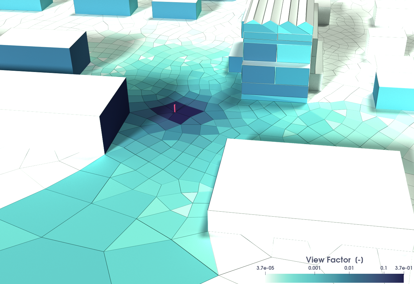
• This library enables the computation of radiation view factors between palanar polygons using an accurate double‐contour integration method described in (Mazumder and Ravishankar 2012) with insights from (Schmid 2016).
• It uses the handy Pyvista package to deal with geometry imports (*.stl, *.vtk, *.obj, ...), geometry creations, and some other mesh functionallities under the hood,
• For a given geometry or set of planar faces, with pyViewFactor you will able to : [x] Optionally check that the faces can "see" each other with get_visibility(face1, face2, ...), [x] Optionally check that no obstruction lies between them with get_obstruction(face1, face2, obstacle, ...), [x] Compute the view factor from face2 to face1 with compute_view_factor(face1, face2, ...), [x] Compute the view factor matrix for a complete mesh, in parallel 🚀, with compute_viewfactor_matrix(mesh, ...)!

[!NOTE] All the examples below are provided as *.py files in the /examples/ folder of the repository, with additional usecases.

Quick Start

Suppose we want to compute the radiation view factor between a triangle and a rectangle facing each other:

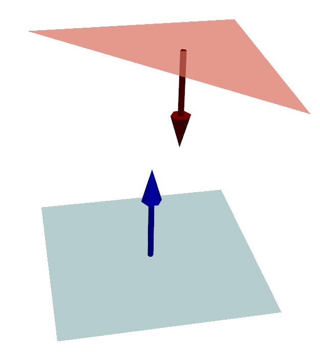
You are few lines of code away from your first view factor computation:

import pyvista as pv
import pyviewfactor as pvf

# Create a rectangle and a triangle facing each other
pointa1 = [0.0, 0.0, 0.0]
pointb1 = [1.0, 0.0, 0.0]
pointc1 = [0.0, 1.0, 0.0]
rectangle = pv.Rectangle([pointa1, pointb1, pointc1])

pointa2 = [0.0, 0.0, 1.0]
pointb2 = [0.0, 1.0, 1.0]
pointc2 = [1.0, 1.0, 1.0]
triangle = pv.Triangle([pointa2, pointb2, pointc2])

if get_visibility(rectangle, triangle):
    F = compute_viewfactor(triangle, rectangle)
    print("VF from rectangle to triangle :", F)
else:
    print("Not facing each other")

pl = pv.Plotter()
pl.add_mesh(rectangle, color="lightblue", opacity=0.7)
pl.add_mesh(triangle, color="salmon", opacity=0.7)

# compute and glyph normals for mesh1
n1 = rectangle.compute_normals(cell_normals=True, point_normals=False)
arrows1 = n1.glyph(orient="Normals", factor=0.1)
pl.add_mesh(arrows1, color="blue")
# similarly for mesh2
n2 = triangle.compute_normals(cell_normals=True, point_normals=False)
arrows2 = n2.glyph(orient="Normals", factor=0.1)
pl.add_mesh(arrows2, color="darkred")

pl.show()

You usually get your geometry from a different format? (*.dat, *.idf, ...)

Check pyvista's documentation on how to generate a PolyData facet from points.

More Examples

Example with a closed geometry and the VTK file format

We will now compute the view factors within a more complex geometry: a closed sphere (clipped in half below), with inwards facing normals, so the faces can "see" each other. Note that the face-to-face visibility is unobstructed (for obstructed geometries, see next section).

The field of view factors from one facet to all others will be computed and stored in a .vtk file, which you can explore with the open source Paraview software.

The following snippet can be reused as a kick-start for your own purposes:

import pyvista as pv
import numpy as np
import pyviewfactor as pvf

sphere = pv.Sphere(radius=10, center=(0, 0, 0), direction=(0, 0, 1),
                   theta_resolution=8, phi_resolution=8,
                   start_theta=0, end_theta=360,
                   start_phi=0, end_phi=180)
# triangulate
sphere.triangulate(inplace=True)
# and put the normals inwards please
# sphere.flip_faces(inplace=True)

# let us chose a cell to compute view factors to
cell_extracted_id = 2
# let us chose a cell to compute view factors to
chosen_face = sphere.extract_cells(cell_extracted_id)
# convert to PolyData
chosen_face = pvf.fc_unstruc2poly(chosen_face)

# "one array to contain them all"
F = np.zeros(sphere.n_cells)
# now let us compute the view factor to all other faces in a sequential way
for i in range(sphere.n_cells):
    if i != cell_extracted_id:
        face = sphere.extract_cells(i)  # other facet
        face = pvf.fc_unstruc2poly(face)  # convert to PolyData
        if pvf.get_visibility(face, chosen_face):
            # compute VF
            F[i] = pvf.compute_viewfactor(face,
                                          chosen_face,
                                          epsilon=0.00001,
                                          rounding_decimal=7)
        else:
            print("Problem, all cells should see each other.")


print("Sum check: \n (is Sum_i^n F_i =? 1)", np.sum(F))

# put the scalar values in the geometry
sphere.cell_data["F"] = F
sphere.save("./sphere.vtk") # ... and save.

# let us have a look in 3D with an interactive window...
pl = pv.Plotter()  # instantiate 3D window
pl.add_mesh(sphere, scalars="VF1", cmap="jet")  # add mesh with a nice color scheme
outline = chosen_face.outline()  # gives you just the wireframe of that cell
pl.add_mesh(
    outline,
    color="red",  # pick a contrasting color
    line_width=3.0,  # thicker line so it stands out
    pickable=False
)
pl.show()

# Alternatively, you can compute the full VF matrix rather easily : 
# Computation of the Fij matrix in parallel
F = pvf.compute_viewfactor_matrix(
    sphere,
    skip_visibility=True,
    skip_obstruction=True,
    compute_kwargs={"epsilon": 1e-4, "rounding_decimal": 8},
    n_jobs=4
)

# We can do the same check as previously for the extracted cell
print("Sum check: \n (is Sum_i^n F_i =? 1)", cell_extracted_id,
      "=", F[:, cell_extracted_id].sum())

The results look as per following images showing the view factor from the chosen cell to all others.

View factors of an individual with a wall

For comfort computations, it may be useful to determine heat transfer between an invidivual and a wall. We will use here PyVista's doorman example as a basis for the human geometry.

The following code and .vtk file of the doorman example are available in the ./examples/ folder.

from tqdm import tqdm
import numpy as np
import pyvista as pv
import pyviewfactor as pvf

def fc_Fwall(nom_vtk):
    # This function is bit more generic than this specific use case,
    # so it can be reused for other applications
    mesh = pv.read(nom_vtk)

    # find all types of walls : in this example only a ground
    wall_types = list(np.unique(mesh["geom_id"]))
    # remove the individual from the list (still named "cylinder"...)
    wall_types.remove("doorman")
    # where is the doorman in the list?
    index_doorman = np.where(mesh["geom_id"] == "doorman")[0]
    # prepare storage for the different walls in a dict
    dict_F = {}
    # loop over wall types
    for type_wall in wall_types:
        # prepare for storing doorman to wall view factor
        F = np.zeros(mesh.n_cells)
        # get the indices of this type of wall
        indices = np.where(mesh["geom_id"] == type_wall)[0]
        # loop over
        for i in indices:
            wall = mesh.extract_cells(i)
            wall = pvf.fc_unstruc2poly(wall)  # convert for normals
            # ... for each facet of the individual
            for idx in tqdm(index_doorman):
                face = mesh.extract_cells(idx)
                face = pvf.fc_unstruc2poly(face)  # convert for normals
                # check if faces can "see" each other
                if pvf.get_visibility(wall, face):
                    # compute face2wall view factor
                    Ffp = pvf.compute_viewfactor(wall, face)
                else:
                    Ffp = 0
                F[idx] = Ffp
        # store array F in e.g. dict_F["F_ceiling"]
        dict_F["F_" + type_wall.replace("\r", "")] = F
    return dict_F

# You can get the  doorman geomtry it directly from here:
# https://gitlab.com/arep-dev/pyViewFactor/-/blob/main/examples/example_doorman_clean.vtk
# ... or get it from this repository's examples
file = "./src_data/example_doorman_clean.vtk"

# compute the VFs for the doorman to the different wall types in the scene
dict_F = fc_Fwall(file)

# re-read and store
mesh = pv.read(file)
# loop over what is in the dictionary of view factors
for elt in dict_F.keys():
    mesh[elt.replace("\r", "")] = dict_F[elt]  # name the field
mesh.save("./src_data/example_doorman_VFground.vtk")  # store in the intial VTK

# have a look without paraview with fancy colors
mesh.plot(cmap="magma_r", lighting=False)

More details and view factors abacuses can be found here.

If you find the computation time a bit lengthy ⌛:

• You can use the compute_viewfactor_matrix() function that leverages joblib with a built-in n_jobs argument 🚀,
• More generally, you can learn how to go parallel here!.

Computing the view factors of a wall in its built environment

For building simulation purposes, it may prove to be useful to compute the ground and sky view factors of a given wall, or the view factor of the wall to other walls in the built environment. In following example (available in the /examples/ folder), we compute the view factors of the environment of the purple wall depicted below.

# Read the geometry
mesh = pv.read("./src_data/built_envmt.vtk")
meshpoly = pvf.fc_unstruc2poly(mesh)  # convert to polydata for obstruction check

# identify who is who
i_wall = np.where(mesh["wall_names"] == "wall")[0]
i_sky = np.where(mesh["wall_names"] == "sky")[0]
i_building1 = np.where(mesh["wall_names"] == "building1")[0]
i_building2 = np.where(mesh["wall_names"] == "building2")[0]

# get the different elements
wall = mesh.extract_cells(i_wall)
sky = mesh.extract_cells(i_sky)
building1 = mesh.extract_cells(i_building1)
building2 = mesh.extract_cells(i_building2)

# convert to polydata
wall = pvf.fc_unstruc2poly(wall)

# Initialize the View Factor
Fsky = 0
# for all cells constituting the ensemble
for patch in tqdm(i_sky):
    sky = mesh.extract_cells(patch)  # extract one cell
    sky = pvf.fc_unstruc2poly(sky)  # convert to polydata
    if pvf.get_visibility(sky, wall, strict=True):
        if pvf.get_obstruction(sky, wall, meshpoly, strict=True):
            # compute and increment view factor :
            # F_i->(j+k) = F_i->j + F_i->k
            Fsky += pvf.compute_viewfactor(sky, wall)

# same for building 1
Fbuilding1 = 0
for patch in tqdm(i_building1):
    bldng1 = mesh.extract_cells(patch)
    bldng1 = pvf.fc_unstruc2poly(bldng1)
    if pvf.get_visibility(bldng1, wall):
        if pvf.get_obstruction(bldng1, wall, meshpoly):
            Fbuilding1 += pvf.compute_viewfactor(bldng1, wall)

# same for building 2
Fbuilding2 = 0
for patch in tqdm(i_building2):
    bldng2 = mesh.extract_cells(patch)
    bldng2 = pvf.fc_unstruc2poly(bldng2)
    if pvf.get_visibility(bldng2, wall):
        if pvf.get_obstruction(bldng2, wall, meshpoly):
            Fbuilding2 += pvf.compute_viewfactor(bldng2, wall)

# complementarity implies \sigma F_i = 1 : compute viewfactor to ground
Fground = 1 - Fbuilding1 - Fbuilding2 - Fsky

# Print results
print("\n-----------------------------")
print("Wall to Sky view factor:")
print("\tSky ", round(Fsky, 4))
print("Wall to Buildings view factors:")
print("\tBuilding 1 ", round(Fbuilding1, 4))
print("\tBuilding 2 ", round(Fbuilding2, 4))
print("Ground view factor:")
print("\tGround ", round(Fground, 4))

The code yields following view factors :

F_{\text{sky}} = 0.345 \\
F_{\text{ground}} = 0.373 \\
F_{\text{building1}} = 0.251 \\
F_{\text{building2}} = 0.031 \\

Understanding the obstruction check function

In real life problems, obstacles may well hinder the radiation heat transfer between surfaces. We thus provide a function to perform obstruction tests, as per following example.

The code snippet below shows how the function get_obstruction() works and allows to understand its usage.

import pyvista as pv
import pyviewfactor as pvf

# let us first create two rectangles

pointa = [0.0, 0.0, 0.0]
pointb = [1.0, 0.0, 0.0]
pointc = [0.0, 1.0, 0.0]
rectangle_down = pv.Rectangle([pointa, pointb, pointc])

pointa = [0.0, 0.0, 1.0]
pointb = [0.0, 1.0, 1.0]
pointc = [1.0, 0.0, 1.0]
rectangle_up = pv.Rectangle([pointa, pointb, pointc])

# a circle will be the obstruction
z_translation, r = 0.5, 2
obstacle = pv.Circle(radius=r, resolution=10)
obstacle.triangulate(inplace=True)
# we translate the obstruction right between both rectangles
obstacle.translate([0, 0, z_translation], inplace=True)
# Define line segment
start = rectangle_down.cell_centers().points[0]
stop = rectangle_up.cell_centers().points[0]
# Perform ray trace
# points, ind = obstacle.ray_trace(start, stop)

# Create geometry to represent ray trace
ray = pv.Line(start, stop)

# Now we can use the get_obtruction function, to check for the obstruction,
# and see each cell of the obstruction mesh is in the way.
obstruction_cell = []
for idx in range(obstacle.n_cells):
    obs = obstacle.get_cell(idx).cast_to_polydata()
    visible = pvf.get_obstruction(rectangle_down, rectangle_up, obs,
                                  strict=False, print_debug=False)
    if not visible[0]:
        print("Cell {} of the obstactle is in the way of the".format(idx)
              + "centroids of rectangle_up and rectangle_down")
        obstruction_cell.append(idx)

obs = obstacle.extract_cells(obstruction_cell)

# if any intersection
if obs.n_cells > 0:
    p = pv.Plotter()
    p.add_mesh(obstacle, show_edges=True, opacity=0.4, color="red",
               lighting=False, label="obstacle")
    p.add_mesh(rectangle_up, color="blue", line_width=5, opacity=0.9,
               label="rect up")
    p.add_mesh(rectangle_down, color="orange", line_width=5, opacity=0.9,
               label="rect down")
    p.add_mesh(ray, color="black", line_width=5, label="ray trace")
    p.add_mesh(obs, show_edges=True, opacity=0.9, color="green", lighting=False,
               label="cell_obstrucion")
    p.add_legend()
    p.show()

Installation

pyViewFactor can be installed from PyPi using pip on Python >= 3.10:

pip install pyviewfactor

You can also visit PyPi or Gitlab to download the sources.

Requirements:

numpy==1.26.4
pyvista==0.45
scipy==1.11.4
numba==0.61.2
joblib==1.2.0
tqdm==4.65.0

The code will probably work with lower versions of the required packages, however this has not been tested.

[!NOTE] If you are alergic to numba, you may pip install pyviewfactor==0.0.10 that works (and give up the times 3+ speed-up in view factor computation).

Citation & Acknowledgments

• Main contributors:
  • Mateusz BOGDAN,
  • Edouard WALTHER.
• Acknowledgment: The authors would like to acknowledge M. Alecian for his initial work on the quadrature code and M. Chapon for her contribution to the code validation.

There is even a conference paper, showing analytical validations.

So if you use pyViewFactor in your work, please cite:

[!IMPORTANT] Citation: Mateusz BOGDAN, Edouard WALTHER, Marc ALECIAN and Mina CHAPON. Calcul des facteurs de forme entre polygones - Application à la thermique urbaine et aux études de confort. IBPSA France 2022, Châlons-en-Champagne.

Bibtex entry:

@inproceedings{pyViewFactor22bogdan,
  authors      = "Mateusz BOGDAN and Edouard WALTHER and Marc ALECIAN and Mina CHAPON",
  title        = "Calcul des facteurs de forme entre polygones - Application à la thermique urbaine et aux études de confort",
  year         = "2022",
  organization = "IBPSA France",
  venue        = "Châlons-en-Champagne, France"
  note         = "IBPSA France 2022",
}

License

MIT License - Copyright (c) AREP 2025