xarray DataArray accessors for PyVista
Project description
PyVista xarray


xarray DataArray accessors for PyVista to visualize datasets in 3D
Usage
Import pvxarray to register the .pyvista accessor on xarray DataArray
and Dataset objects. This gives you access to methods for creating 3D meshes,
plotting, and lazy evaluation of large datasets.
Try on MyBinder: https://mybinder.org/v2/gh/pyvista/pyvista-xarray/HEAD
import pvxarray
import xarray as xr
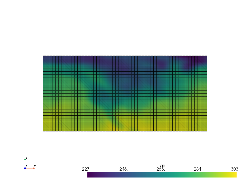
ds = xr.tutorial.load_dataset("air_temperature")
da = ds.air[dict(time=0)]
# Plot in 3D
da.pyvista.plot(x="lon", y="lat", show_edges=True, cpos='xy')
# Or grab the mesh object for use with PyVista
mesh = da.pyvista.mesh(x="lon", y="lat")
Coordinate Auto-Detection
If your data follows CF conventions, you can
omit the x, y, and z arguments entirely. pyvista-xarray uses
cf-xarray to detect coordinate axes
from attributes like axis, standard_name, and units, as well as
variable name heuristics:
import pvxarray
import xarray as xr

ds = xr.tutorial.load_dataset("air_temperature")
da = ds.air[dict(time=0)]

# Coordinates are auto-detected from CF attributes
mesh = da.pyvista.mesh()

# Inspect the detected axes
da.pyvista.axes
# {'X': 'lon', 'Y': 'lat'}
Lazy Evaluation with Algorithm Sources
For large or dask-backed datasets, create a VTK algorithm source that lazily evaluates data on demand. This avoids loading the entire dataset into memory and supports time stepping, resolution control, and spatial slicing:
import pvxarray
import pyvista as pv
import xarray as xr

ds = xr.tutorial.load_dataset("air_temperature")
da = ds.air

# Create a lazy algorithm source with time stepping
source = da.pyvista.algorithm(x="lon", y="lat", time="time")

# Add directly to a plotter
pl = pv.Plotter()
pl.add_mesh(source)
pl.show(cpos="xy")

# Step through time
source.time_index = 10
Use the resolution parameter to downsample large datasets for interactive
rendering:
source = da.pyvista.algorithm(x="lon", y="lat", time="time", resolution=0.5)
Algorithm sources also expose human-readable time labels from datetime coordinates:
source.time_label # e.g. '2013-01-01 00:00:00'
Dataset Accessor
The .pyvista accessor also works on Dataset objects, letting you load
multiple data variables onto a single mesh. This is useful when a dataset
contains several fields (e.g. wind components, temperature, pressure) that
share the same grid:
import pvxarray
import xarray as xr

ds = xr.tutorial.load_dataset("eraint_uvz")

# Discover which variables share the same dimensions
ds.pyvista.available_arrays()
# ['z', 'u', 'v']

# Create a mesh with all three variables as point data
mesh = ds.pyvista.mesh(
    arrays=["u", "v", "z"],
    x="longitude",
    y="latitude",
)

# Or create a lazy algorithm source for large datasets
source = ds.pyvista.algorithm(
    arrays=["u", "v"],
    x="longitude",
    y="latitude",
    z="level",
    time="month",
)
Computed Fields
Derive new arrays on the fly with vtkArrayCalculator expressions. This is
useful for computing quantities like wind speed from vector components without
modifying the underlying dataset:
import pvxarray
import xarray as xr

ds = xr.tutorial.load_dataset("eraint_uvz")

source = ds.pyvista.algorithm(
    arrays=["u", "v"],
    x="longitude",
    y="latitude",
    z="level",
    time="month",
)

# Add a derived wind speed field
source.computed = {
    "_use_scalars": ["u", "v"],
    "wind_speed": "sqrt(u*u + v*v)",
}
Expressions follow vtkArrayCalculator syntax and can reference any array
loaded onto the mesh.
Pipeline Extensibility
Inject post-processing filters into the source's evaluation chain. Each element can be a VTK algorithm or a callable that takes and returns a PyVista mesh:
# Apply a warp filter after mesh creation
source.pipeline = [lambda mesh: mesh.warp_by_scalar(factor=0.001)]
Filters run in order after computed fields are evaluated and the result is passed downstream to the plotter.
State Serialization
Save and restore source configurations as JSON for reproducible visualizations:
# Save the current configuration
config = source.to_json()

# Later, recreate the source with the same settings
restored = PyVistaXarraySource.from_json(
    config,
    data_array=ds["u"],
    dataset=ds,
)
The state captures coordinate mappings, time index, resolution, array selections, and computed field definitions.
Reading VTK Files as xarray Datasets
Read VTK mesh files directly into xarray using the pyvista backend
engine. Supported formats include .vti, .vtr, .vts, and .vtk:
import xarray as xr

ds = xr.open_dataset("data.vtk", engine="pyvista")
ds["data array"].pyvista.plot(x="x", y="y", z="z")
Converting PyVista Meshes to xarray
Convert PyVista meshes back to xarray Datasets with pyvista_to_xarray.
Supported mesh types: RectilinearGrid, ImageData, and StructuredGrid:
import pyvista as pv
from pvxarray import pyvista_to_xarray

grid = pv.RectilinearGrid([0, 1, 2], [0, 1], [0, 1])
grid["values"] = range(grid.n_points)
ds = pyvista_to_xarray(grid)
Installation
pip install 'pyvista-xarray[jupyter]'
This includes Jupyter rendering support (via Trame), common I/O libraries
(netcdf4, rioxarray), and dask for lazy evaluation. For a minimal
install without these extras:
pip install pyvista-xarray
pyvista-xarray is also available on conda-forge:
conda install -c conda-forge pyvista-xarray
Examples
The examples/
directory contains Jupyter notebooks demonstrating various use cases:
| Notebook | Description |
|---|---|
| introduction.ipynb | Quick start with auto-detection, rioxarray, and 3D grids |
| simple.ipynb | Lazy evaluation, time stepping, and algorithm sources |
| ocean_model.ipynb | Curvilinear grids with ROMS ocean model data |
| atmospheric_levels.ipynb | 3D atmospheric data across pressure levels |
| lightning.ipynb | Point cloud visualization from scattered observations |
| cartographic.ipynb | Geographic projections with GeoVista |
| radar.ipynb | Radar data with polar coordinates via xradar |
| sea_temps.ipynb | Sea surface temperature raster data |
There are also Python scripts for interactive Trame web applications:
examples/level_of_detail.py and examples/level_of_detail_geovista.py.
Simple RectilinearGrid
import numpy as np
import pvxarray
import xarray as xr

lon = np.array([-99.83, -99.32])
lat = np.array([42.25, 42.21])
z = np.array([0, 10])
temp = 15 + 8 * np.random.randn(2, 2, 2)

ds = xr.Dataset(
    {
        "temperature": (["z", "x", "y"], temp),
    },
    coords={
        "lon": (["x"], lon),
        "lat": (["y"], lat),
        "z": (["z"], z),
    },
)

mesh = ds.temperature.pyvista.mesh(x="lon", y="lat", z="z")
mesh.plot()
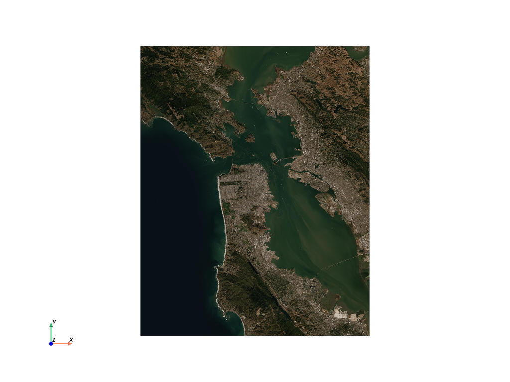
Raster with rioxarray
import pvxarray
import rioxarray
import xarray as xr

da = rioxarray.open_rasterio("TC_NG_SFBay_US_Geo_COG.tif")
da = da.rio.reproject("EPSG:3857")

# Grab the mesh object for use with PyVista
mesh = da.pyvista.mesh(x="x", y="y", component="band")

mesh.plot(scalars="data", cpos='xy', rgb=True)
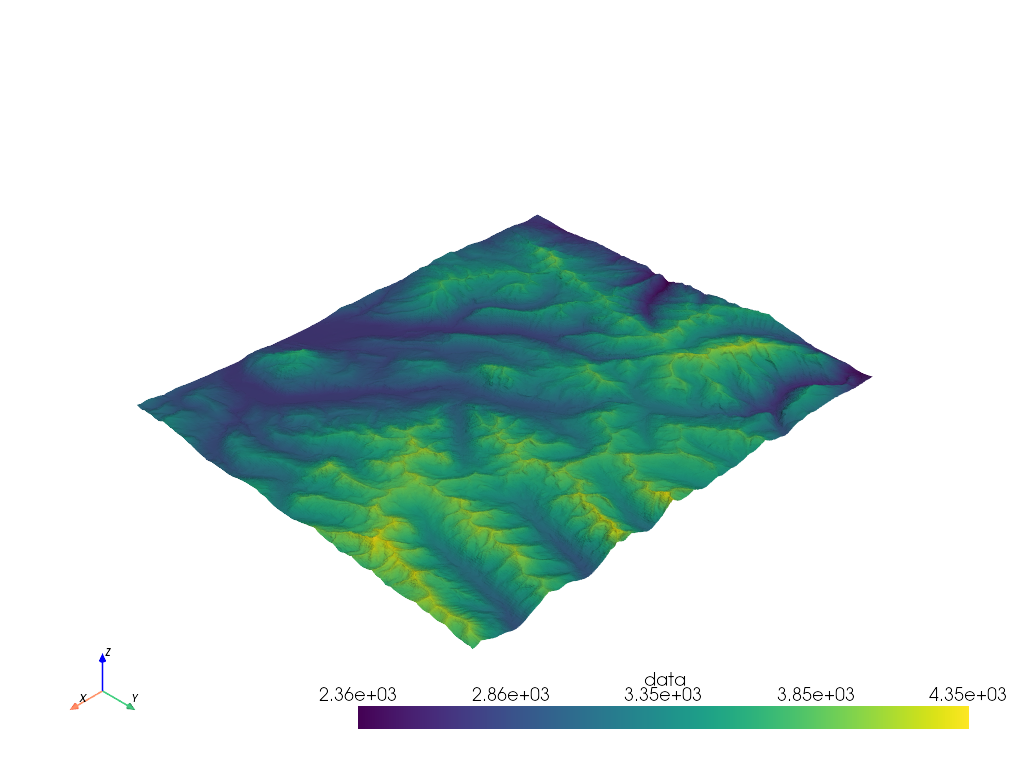
import pvxarray
import rioxarray

da = rioxarray.open_rasterio("Elevation.tif")
da = da.rio.reproject("EPSG:3857")

# Grab the mesh object for use with PyVista
mesh = da.pyvista.mesh(x="x", y="y")

# Warp top and plot in 3D
mesh.warp_by_scalar().plot()
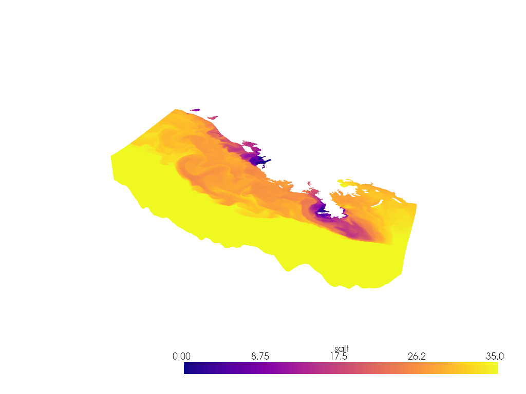
StructuredGrid
import pvxarray
import pyvista as pv
import xarray as xr

ds = xr.tutorial.open_dataset("ROMS_example.nc", chunks={"ocean_time": 1})

if ds.Vtransform == 1:
    Zo_rho = ds.hc * (ds.s_rho - ds.Cs_r) + ds.Cs_r * ds.h
    z_rho = Zo_rho + ds.zeta * (1 + Zo_rho / ds.h)
elif ds.Vtransform == 2:
    Zo_rho = (ds.hc * ds.s_rho + ds.Cs_r * ds.h) / (ds.hc + ds.h)
    z_rho = ds.zeta + (ds.zeta + ds.h) * Zo_rho

ds.coords["z_rho"] = z_rho.transpose()  # needing transpose seems to be an xarray bug

da = ds.salt[dict(ocean_time=0)]

# Make array ordering consistent
da = da.transpose("s_rho", "xi_rho", "eta_rho", transpose_coords=False)

# Grab StructuredGrid mesh
mesh = da.pyvista.mesh(x="lon_rho", y="lat_rho", z="z_rho")

# Plot in 3D
p = pv.Plotter()
p.add_mesh(mesh, lighting=False, cmap='plasma', clim=[0, 35])
p.view_vector([1, -1, 1])
p.set_scale(zscale=0.001)
p.show()
Feedback
Please share your thoughts and questions on the Discussions board. If you would like to report any bugs or make feature requests, please open an issue.
If filing a bug report, please share a scooby Report:
import pvxarray
print(pvxarray.Report())
Project details
Release history Release notifications | RSS feed


Download files
Download the file for your platform. If you're not sure which to choose, learn more about installing packages.
Source Distribution
Built Distribution
Filter files by name, interpreter, ABI, and platform.
If you're not sure about the file name format, learn more about wheel file names.
Copy a direct link to the current filters
File details
Details for the file pyvista_xarray-0.2.0.dev0.tar.gz.
File metadata
- Download URL: pyvista_xarray-0.2.0.dev0.tar.gz
- Upload date:
- Size: 39.4 kB
- Tags: Source
- Uploaded using Trusted Publishing? No
- Uploaded via: twine/6.2.0 CPython/3.12.12
File hashes
| Algorithm | Hash digest | |
|---|---|---|
| SHA256 |
647410a990263f62f7ed589c3e424629b51527879b49953f754e0d8df6f574bd
|
|
| MD5 |
58e3ddca8a1fd640e8098c5ce759277d
|
|
| BLAKE2b-256 |
732fd4539cea6945eebf47cff656138e3e02456fdf8bf9c182a195f3b1e469ab
|
File details
Details for the file pyvista_xarray-0.2.0.dev0-py3-none-any.whl.
File metadata
- Download URL: pyvista_xarray-0.2.0.dev0-py3-none-any.whl
- Upload date:
- Size: 32.9 kB
- Tags: Python 3
- Uploaded using Trusted Publishing? No
- Uploaded via: twine/6.2.0 CPython/3.12.12
File hashes
| Algorithm | Hash digest | |
|---|---|---|
| SHA256 |
25c626f6cd96157a688489d33f877001b4dc1c8384f246d255b44fb1e6e6c908
|
|
| MD5 |
6015855c5f0cb20e7ebbdcafbc692303
|
|
| BLAKE2b-256 |
6ebc1d8bedd9f97ec292df73ee01d6e07558d5e90e8391bfda24512ddebdc75a
|


