
QASP




QASP (Quantum Agent Software Package) is a Python toolkit for building, training and analyzing quantum models with PennyLane and PyTorch. Shared circuit builders, feature maps, ansatz templates and initializers support reinforcement learning, classification, quantum kernels, generative learning and combinatorial optimization.
Run compatible models with PennyLane devices or QASP's differentiable IQPSimulator (tensor networks, Van den Nest estimation or automatic selection) and PauliPropagationSimulator. Reuse the same building blocks across modules, with execution and gradient methods chosen for each circuit and readout.
Get started · Tutorials · Examples · Documentation website · Package guide · Architecture
Table of contents
- Highlights
- Architecture
- Documentation
- Installation
- Dependencies
- Differentiable IQP simulation
- General differentiable Pauli propagation
- Package layout
- Top-level API
- Distributed statevector simulation (MPI)
- Manual circuit construction example
- High level RL policies from dictionaries and
create_model - Reinforcement learning example with REINFORCE
- Policy classes in
qasp.rl.policies - Trainability and analysis utilities
- Notebooks and example scripts
- End-to-end CartPole examples
- Citing QASP
Highlights
- Build PQCs from composable feature maps and ansätze
- Train Born and softmax policies on Gym/Gymnasium-style environments
- Run lightweight REINFORCE training loops directly from QASP
- Evaluate trainability with utilities such as:
- model-agnostic cost-concentration diagnosis,
- policy variance,
- exploratory Lie-closure dimensions (with documented heuristic limitations)
- Use PennyLane lightning.qubit / lightning.kokkos and the shared differentiable PauliPropagationSimulator (legacy
lightning.ppremains available) - Run differentiable commuting models with IQPSimulator: exact TN, sampled Van den Nest, or automatic selection, with multicore forward/backward execution
- Compare different observable/readout designs, including local
Z, pairwiseZZ, and parity-based observables - Build global-fidelity, local-fidelity, and projected quantum kernels, including trainable IQP encodings
- Optimize trainable kernels with centered kernel-target alignment
- Train binary and multiclass PQC classifiers with MSE, hinge, binary cross-entropy, or categorical cross-entropy
- Decode Born probabilities into classes with contiguous, parity, or majority partitions
- Evaluate classifiers with accuracy, balanced accuracy, precision, recall, F1, ROC AUC, PR AUC, confusion matrices, log loss, and Brier score
- Solve QUBOs with standard, multi-angle, warm-start, recursive, and linear-ramp QAOA
- Define custom QAOA mixers and PCE parameterized circuits with QASP dictionaries
- Export paper-ready circuit drawings as editable TikZ/Quantikz, with symbolic parameters, gate colors, and repeated-layer compression
Architecture
Feature maps (AngleEmbedding, NeuralEmbedding) supply input encoding to
ansatz templates (AngleAnsatz, IQPAnsatz). CircuitBuilder combines the
ansatz with a measurement and compiles it into a QNode, optionally wrapped in a
trainable TorchLayer. Initializers configure circuit weights and input scales;
the shared device layer selects a compatible simulator. These components support
RL, classifiers, kernels, optimization and generative learning.

Editable vector diagram · PNG · Rendering source
This is a conceptual dependency view. QAOA constructs cost/mixer QNodes directly
and shares device selection; PCE can use CircuitBuilder. Backend compatibility
still depends on the circuit, measurement and differentiation method. Full
initializer options are listed under parameter initialization.
Documentation
The module tutorials are runnable Jupyter notebooks covering circuit construction, training, results, Matplotlib and TikZ drawings, trainability diagnostics and differentiable simulation.
In Jupyter, tex = draw_classifier(model, inputs=x, output="tikz") previews
the circuit and returns its LaTeX. Pass return_tex=False for a preview only.
The same convention applies across module drawing helpers.
See the drawing guide
for optional rendering dependencies and examples.
Explore the interactive QASP documentation: Building Blocks → Simulators → Modules, with step-by-step configuration, training and visualization examples, searchable APIs and argument descriptions.
This repository contains the library, regression tests and a curated example set. Notebook outputs, experiment datasets and paper sources/PDFs are kept in the upstream research archive. See the repository layout policy for what is retained and how to keep the checkout small.
Start with the package guide for the complete module
map, executable examples, data shapes and implementation boundaries, alongside
the package’s module and API docstrings.
The documentation audit records verification and
environment limitations. Focused guides cover Q-functions
and generative learning. The unified IQP guide
explains IQPSimulator, exact TN versus sampled VN, gradients, automatic selection
and resource limits. Start with the IQP tutorial
or parallel-gradient neural-policy example.
The QASP software paper includes
selected IQP experiments and the shared Pauli simulator’s mathematics, limitations
and validated application examples. The Pauli-propagation guide
covers configuration and migration; the dedicated IQP paper
contains the full mathematical and performance study.
Installation
QASP 0.1.3 is an alpha research release. It requires Python 3.10 or newer, subject to dependency support; Python 3.12 is a tested starting point.
From PyPI
Create an isolated environment, then install the published package:
python3.12 -m venv .venv
source .venv/bin/activate
python -m pip install --upgrade pip
python -m pip install qasp
python -m pip check
python -c "from importlib.metadata import version; import qasp; print(version('qasp'))"
For a reproducible package version, use python -m pip install qasp==0.1.3.
The package includes its core Python dependencies. Optional PennyLane device
plugins, GPU/MPI libraries and tensor-device dependencies require separate
installation appropriate to your platform. See the
device and compilation guide.
From source
git clone https://github.com/INESCTEC/qasp.git
cd qasp
python -m pip install -e .
Development install
python -m pip install -e .[dev]
Dependencies
QASP relies primarily on:
pennylanetorchnumpyscipyautogradopt_einsum(exact IQP contraction)gymnasiumtorchrltensordictmatplotlibpandasray[rllib]
The tested dependency ranges are in pyproject.toml. See the
compatibility matrix for Python 3.10–3.12
results on macOS arm64, reproducible version constraints and known limitations.
Each of four clean profiles passes 746 tests, with three optional Kokkos tests
skipped; the reference torchlane environment passes all 749 tests.
PennyLane tensor-network comparison experiments additionally use quimb;
QASP's IQP TN route uses opt_einsum.
Differentiable IQP simulation
IQPSimulator executes compatible commuting quantum models through one device:
backend |
Computation | Suitable readouts |
|---|---|---|
"tn" |
Exact tensor-network contraction with Torch gradients | Supported moments and structured Born/action probabilities |
"van_den_nest" |
Differentiable Monte Carlo correlation estimates | Real I/Z expectations; optional compact projector importance sampling |
"auto" (default) |
Chooses an eligible route using resource estimates | Depends on the circuit, readout and approximation budget |
The shared construction is a circuit of commuting X-string rotations on
|0...0>, or its equivalent closed Hadamard-frame Z circuit. RX, RXX and RXXX
AngleAnsatz layers and matching-axis feature encodings are examples.
IQPAnsatz configurations must also satisfy the circuit/readout contract;
arbitrary noncommuting gates are not made eligible by the device name.
TN accepts a broader recognized product-basis circuit family.
This complete example constructs a QASP policy directly: the configuration
selects the commuting ansatz, neural embedding, observables and IQP backend.
PQCSoftmax returns logits, so the training loss applies log_softmax to form
action log-probabilities.
import numpy as np
import torch
from qasp import AngleAnsatz, NeuralEmbedding
from qasp.rl.policies import PQCSoftmax

n = 8
config = {
    "ansatz": AngleAnsatz,
    "ansatz_config": {
        "n_qubits": n, "n_layers": 2,
        "rotations": ([f"X {w}" for w in range(n)]
                      + [f"XX {w} {w+1}" for w in range(n-1)]
                      + [f"XXX {w} {w+1} {w+2}" for w in range(n-2)]),
        "include_imprimitive": False,
        "include_hadamards_initial": False, "reuploading": True,
    },
    "feature_map": NeuralEmbedding,
    "feature_map_config": {"n_qubits": n, "features": 4,
                           "rotations": "X"},
    "n_actions": 2, "observables": ["Z 0", f"Z {n-1}"],
    "fc_layer": None,
    "device": "IQPSimulator",
    "device_kwargs": {"backend": "auto", "mode": "explicit",
                      "vn_samples": 4096, "vn_workers": 4,
                      "vn_parallel_backward": True, "seed": 2026},
    "diff_method": "backprop", "shots": None,
}
policy = PQCSoftmax(n_qubits=n, **config).double()
x = torch.tensor(np.array([.2, -.4, .3, .1]), dtype=torch.float64,
                 requires_grad=True)
optimizer = torch.optim.Adam(policy.parameters(), lr=.01)
optimizer.zero_grad()
loss = -torch.log_softmax(policy(x), dim=-1)[1]
loss.backward()
assert torch.isfinite(x.grad).all()
assert all(p.grad is not None and torch.isfinite(p.grad).all()
           for p in policy.parameters())
optimizer.step()  # Updates circuit and neural-embedding parameters.
print(policy.circuit.device.last_report.selected)
Change config["device_kwargs"]["backend"] before constructing the policy
to "tn", "van_den_nest", or "auto". The same device fields can be used
in compatible QASP model-factory dictionaries. No hand-written circuit or
QNode is required.
Gradients propagate through shared circuit parameters, inputs, observable coefficients and compatible neural embeddings. This supports IQP-based RL policies, expectation classifiers, projected kernels, generative moment-MMD and compatible optimization circuits. Probability-based majority policies use TN; generic QAOA circuits and arbitrary readouts are not VN workloads. See the public-model tutorial for complete configurations and the parallel-gradient neural-policy example for Adam training.
VN estimates have sampling error even with shots=None; its classical samples
are not quantum-output samples. vn_samples, vn_error and vn_confidence
control additive expectation accuracy, not nonlinear-loss or gradient error.
Use allow_approximate=False or backend="tn" for exact execution.
mode="explicit" disables the separate small-statevector fallback while
retaining automatic TN/VN selection. last_report exposes choices, estimates
and uncertainty. auto is a heuristic, not a guarantee of the fastest backend.
CPU chunk workers parallelize both forward and backward. Effective
concurrency is bounded by the number of sample chunks; numerical thread pools
should be configured at application level to avoid oversubscription.
The worker default is one, and this backend does not implement MPI or
multi-node execution. Higher derivatives are supported on tested eager Torch
paths, with additional memory for retained derivative graphs.
IQPTNSimulator remains available as the exact-only compatibility interface.
The unified guide describes contracts, importance sampling and selection controls. The CPU benchmark report compares previous/new gradient scheduling and 1–8 workers. The IQP research paper contains the TN/VN/PennyLane comparison through 100 qubits, including startup, gradients, resource stops and accuracy qualifications. Selected results are also included in the QASP software paper. These are measured CPU workloads, not universal speedup or equal-accuracy claims.
General differentiable Pauli propagation
PauliPropagationSimulator lives in qasp.simulators alongside IQPSimulator
and is also exported from qasp. It handles noncommuting circuits through
Clifford and arbitrary Pauli-rotation propagation, with exact execution by default.
Use the same device fields in RL, classifiers, kernels, generative learning and
optimization:
execution = {
    "device": "PauliPropagationSimulator",
    "device_kwargs": {"k": None, "prune": False},
    "diff_method": "backprop",
    "shots": None,
}
For example, construct and train a noncommuting neural policy directly through
qasp.rl.policies using that execution dictionary:
import numpy as np
import torch
from qasp import AngleAnsatz, NeuralEmbedding
from qasp.rl.policies import PQCSoftmax

policy = PQCSoftmax(
    n_qubits=3, n_actions=2,
    ansatz=AngleAnsatz,
    ansatz_config={
        "n_qubits": 3, "n_layers": 2,
        "rotations": ["Y 0", "Z 1", "X 2", "XYZ 0 1 2"],
        "include_imprimitive": True, "imprimitive": "CNOT",
        "imprimitive_pattern": "chain", "reuploading": True,
    },
    feature_map=NeuralEmbedding,
    feature_map_config={"n_qubits": 3, "features": 2, "rotations": "Y"},
    observables=["Z 0", "XZ 1 2"], fc_layer=None, **execution,
).double()
x = torch.tensor(np.array([.2, -.4]), dtype=torch.float64, requires_grad=True)
optimizer = torch.optim.Adam(policy.parameters(), lr=.01)
optimizer.zero_grad()
loss = -torch.log_softmax(policy(x), dim=-1)[1]
loss.backward()  # Circuit parameters, neural embedding and inputs share the graph.
assert torch.isfinite(x.grad).all()
assert all(p.grad is not None and torch.isfinite(p.grad).all()
           for p in policy.parameters())
optimizer.step()
| Application | Supported analytic paths |
|---|---|
| RL | Observable policies, Born policies and PQDQN; neural PQDQN inputs use sequential batching. |
| Classifiers | Expectation scores and Born probabilities with Torch training. |
| Kernels | Global/local fidelity projectors and projected Pauli kernels, including trainable Gram matrices. |
| Generative learning | Expectation-based MMD and probability-based NLL; sampling uses an explicitly selected sampling device. |
| Optimization | Torch QAOA and PCE, including multilayer noncommuting circuits. |
The complete direct-QASP example trains
a neural policy and exercises PQDQN, a classifier, a fidelity kernel, MMD, QAOA
and PCE with this configuration. Use backend="torch" for optimization. Torch
gradients include circuit parameters, inputs, neural embeddings and observable
coefficients; analytic expectations, variances and probabilities are supported.
Run the application example with:
conda run -n torchlane python examples/pauli_propagation_modules.py
The public imports are from qasp import PauliPropagationSimulator and
from qasp.simulators import PauliPropagationSimulator. QASP accepts the class,
a configured instance, or the device name shown above. These names are resolved
by QASP, rather than registered as external PennyLane plugins.
Exact Pauli expansions can grow exponentially. Dense probabilities require
2**m moments for m measured wires and default to a 16-wire readout limit.
Optional weight truncation/coefficient pruning changes both outputs and
gradients. Finite shots, noise, amplitude-vector StatePrep, statevector outputs
and MPI are unsupported. Supported unitary templates are decomposed into native
Clifford/Pauli rotations; unsupported operations raise an error. Scalar tapes
are evaluated sequentially, with no dedicated worker pool.
Existing lightning.pp adapters and old engine imports remain compatible;
see the algorithm, module coverage and migration guide.
Package layout
qasp/
├── circuits/
│   ├── constructor.py      # CircuitBuilder and compilation utilities
│   ├── templates.py        # Ansatz templates such as IQPAnsatz and AngleAnsatz
│   ├── tikz.py             # Quantikz/TikZ circuit export
│   └── uqc.py              # Historical circuit prototype (see limitations)
├── feature_maps/
│   └── templates.py        # AngleEmbedding and NeuralEmbedding
├── genlearn/
│   ├── models.py           # PQCBM training and device sampling
│   ├── factory.py          # Dictionary-based create_qcbm
│   ├── drawing.py          # draw_qcbm / Quantikz export
│   └── losses.py           # NLL and expectation-mixture MMD
├── qkernels/
│   ├── kernels.py          # Fisher-information kernel utilities
│   ├── quantum_kernels.py  # Fidelity, local-fidelity, and projected kernels
│   ├── factory.py          # Configuration-driven kernel construction
│   ├── kta.py              # Kernel-target alignment
│   └── use_cases/          # Kernel experiments and examples
├── classifiers/
│   ├── models.py           # PQCClassifier expectation/Born readouts
│   ├── decoders.py         # Contiguous, parity, and majority class decoders
│   ├── losses.py           # MSE, hinge, BCE, and categorical CE
│   ├── metrics.py          # Classification evaluation metrics
│   ├── training.py         # Compact PyTorch training/evaluation loop
│   └── factory.py          # create_classifier configuration factory
├── optimization/
│   ├── problem.py          # QUBO model and QUBO-to-Ising conversion
│   ├── qaoa.py             # standard, multi-angle, warm-start, and LR-QAOA
│   ├── recursive.py        # recursive QAOA elimination and reconstruction
│   ├── pce.py              # Pauli Correlation Encoding with QASP ansätze
│   └── optimizers.py       # reusable SciPy optimizer adapters
├── simulators/             # IQPSimulator, PauliPropagationSimulator and shared engines
├── diagnostics/
│   └── barren_plateau.py   # classifier/kernel/policy cost concentration
├── devices.py              # Shared device/MPI option handling
├── initialization.py       # Reusable NumPy/Torch parameter distributions
└── rl/
    ├── model.py            # create_model, draw_model
    ├── policies.py         # PQCBorn, PQCSoftmax, related policy classes
    ├── metrics.py          # Legacy probability variance / heuristic Lie closure
    ├── pp_sim.py           # truncated Pauli propagation simulator
    ├── differentiable_pp_sim.py
    ├── torchrl.py          # DQN, REINFORCE, PPO, bandits and TorchRL adapter
    ├── qfunctions/         # PQDQN models, Pauli readouts and drawings
    ├── envs.py             # Windy target-navigation environment
    └── trl.py              # Historical TorchRL prototype (see limitations)

examples/                   # Curated tutorials and supporting scripts

tests/
├── test_*.py               # Runtime/API regression tests
└── tests_deucalion/        # Cluster scripts and MPI smoke checks
Top-level API
The package re-exports the most common entry points from qasp.__init__.
Parameter initialization
Use reusable distributions from qasp.initialization to initialize ansatz
weights and feature-map input scales independently:
from qasp import create_classifier
from qasp.initialization import Normal, Uniform

config = {
    "feature_map": "AngleEmbedding",
    "feature_map_config": {"rotations": "Y", "input_scaling": True},
    "ansatz": "AngleAnsatz",
    "ansatz_config": {"n_layers": 2, "rotations": "YZ", "reuploading": True},
    "init": Normal(mu=0.0, std=0.2),
    "input_scaling_init": Uniform(low=0.8, high=1.2),
    "device": "default.qubit",
}
classifier = create_classifier(config, n_qubits=4, n_classes=2)
The same init and input_scaling_init settings work with create_model,
create_qfunction, trainable create_kernel models, and create_qcbm.
They apply to every reuploading layer and to NeuralEmbedding projection
weights. Classical output heads keep their existing initialization.
Available specifications are Normal(mu, std), Uniform(low, high),
Beta(alpha, beta, low=0, high=1), TruncatedNormal(mu, std, low, high),
LogNormal(mu, std), Gamma(concentration, rate), Exponential(rate),
Laplace(mu, scale), Rademacher(scale=1), Constant(value), Zeros(),
Ones(), and Choice(values). Normal.std means
standard deviation. Specifications are immutable and can be reused across
models; each construction draws fresh weights. Legacy strings such as
"normal_0_1" and "random_-pi_pi" still work. Unknown names raise an error.
Suggested starting points (compare them on your circuit and data):
| Goal | Initializer | Why try it |
|---|---|---|
| Small ansatz rotations | Normal(0, 0.1) |
Simple centered baseline |
| Small rotations with strict bounds | TruncatedNormal(0, 0.1, -0.2, 0.2) |
Samples a conditioned normal without clipping values at the endpoints |
| Bounded, center-concentrated angles | Beta(2, 2, low=-0.3, high=0.3) |
Controls concentration as well as range |
AngleEmbedding input scales near one |
Beta(5, 5, low=0.8, high=1.2) |
Mean one with a fixed allowed interval |
| Positive scales with mean one | LogNormal(-0.005, 0.1) or Gamma(100, 100) |
Positive alternatives without a hard upper bound |
Signed NeuralEmbedding projections |
Normal(0, 1 / np.sqrt(n_features)) |
A variance-based starting point for standardized, roughly independent features |
| Equal-magnitude random signs | Rademacher(0.1) |
Discrete symmetric weights |
| Sharper center with occasional larger values | Laplace(0, 0.1) |
Heavier tails than a normal distribution |
| Positive values concentrated near zero | Exponential(rate=10) |
Mean 0.1; useful when that asymmetric start is intentional |
There is no universally best distribution, and small rotations alone do not
guarantee good gradients. For a first comparison, use small Normal versus
TruncatedNormal angles, with Beta or Ones() for AngleEmbedding scales.
NeuralEmbedding scales are projection weights, so a centered distribution is
usually a more useful starting point there. Xavier/Kaiming initializers depend
on a neural layer's fan-in/fan-out and activation; QASP's flat angle vectors
do not contain that structure (PyTorch initialization reference).
Beta's alpha and beta must be positive: equal values above one concentrate
near the midpoint, values below one favor the ends, and unequal values skew
the distribution (NumPy Beta reference).
TruncatedNormal's bounds are actual parameter values; mu and std describe
the underlying normal before truncation (SciPy reference).
LogNormal's mu and std are in log space, Gamma uses rate rather than
scale, and Laplace's standard deviation is sqrt(2) * scale.
from qasp.initialization import Beta, TruncatedNormal

config["init"] = TruncatedNormal(mu=0, std=0.1, low=-0.2, high=0.2)
config["input_scaling_init"] = Beta(alpha=5, beta=5, low=0.8, high=1.2)
classifier = create_classifier(config, n_qubits=4, n_classes=2)
The initialized quantum weights remain trainable PyTorch parameters. For example, continue with the classifier above and update both parameter groups with Adam:
import torch

torch.manual_seed(7)  # Set before constructing the model for reproducible weights.
classifier = create_classifier(config, n_qubits=4, n_classes=2)
optimizer = torch.optim.Adam(classifier.parameters(), lr=0.01)
inputs = torch.tensor([[0.2, -0.3, 0.1, 0.4], [-0.1, 0.5, 0.2, -0.4]])
targets = torch.tensor([0, 1])

optimizer.zero_grad()
loss = classifier.compute_loss(inputs, targets, objective="cross_entropy")
loss.backward()
optimizer.step()
Initialization runs only at construction, not on every optimizer step.
PQCBM uses interface="torch" by default; QAOA and PCE use
backend="torch" for Torch optimization.
CircuitBuilder.create_torchlayer uses initialization=Normal(...) and
input_scaling_init=Uniform(...). Explicit params and
input_scaling_params arrays override only their own group. If no scale
initializer is supplied, Torch layers use the ansatz initializer for both
groups; PQCBM preserves its default input scales of one. Supplying a scale
initializer requires an input-scaling feature map. Encoding-only kernels
can use it to sample fixed scales once.
Optimization models accept the same objects at construction or at solve time:
from qasp import QAOA, QUBO
from qasp.initialization import Normal, Uniform

problem = QUBO.maxcut(3, [(0, 1), (1, 2), (0, 2)])
solver = QAOA(problem, n_layers=2, init=Normal(0.0, 0.15), seed=7)
angles = solver.initial_parameters()  # Uses the constructor's initializer.
result = solver.solve(initial_parameters=Uniform(-0.2, 0.2))  # Optional override.
This also applies to multi-angle QAOA, warm-start QAOA, PCE, and RQAOA's
subproblem solvers. They have no input-scaling parameter group. LR-QAOA keeps
its deterministic schedule, configured by delta_gamma and delta_beta.
The concentration diagnoser accepts initialization=Normal(...) plus
input_scaling_init=... for independent resampling.
Seed Torch before constructing Torch-layer models with torch.manual_seed.
PQCBM, QAOA and PCE use their local seed for built-in distributions;
diagnostics use their local seeded generator. Explicit-parameter APIs such
as QFKernel can use Normal(...).sample(shape, rng=np.random.default_rng(7)).
Torch-style custom callables are also accepted and control their own randomness.
NumPy and Torch use different RNG algorithms, so equal seeds do not imply
identical samples across backends.
Beta, Gamma, Laplace and TruncatedNormal use a local CPU sampler seeded from
Torch's RNG when filling tensors, then copy values to the target dtype/device.
A supplied torch.Generator controls this without changing either global RNG.
The other built-in distributions use native Torch fills. This sampling happens
only during initialization; the resulting model parameters remain trainable.
See the cross-module initialization notebook
for creation, gradients, training, reproducibility and compatibility checks.
Use Choice((0, np.pi / 2)) for explicit discrete values: the historical
"discrete_0_pi_over_2" alias retains its old 0/pi meaning in the builder
and its 0/pi-over-2 meaning in diagnostics.
Circuits
CircuitBuilderIQPAnsatzAngleAnsatzUQC
Feature maps
AngleEmbeddingNeuralEmbedding
Generative learning
PQCBM,create_qcbm,draw_qcbm,PauliMMDBornMachine(deprecated compatibility wrapper)
See the generative-learning guide and the runnable PQCBM notebook for expectation-based MMD, differentiable Pauli propagation, sampling, and MPI.
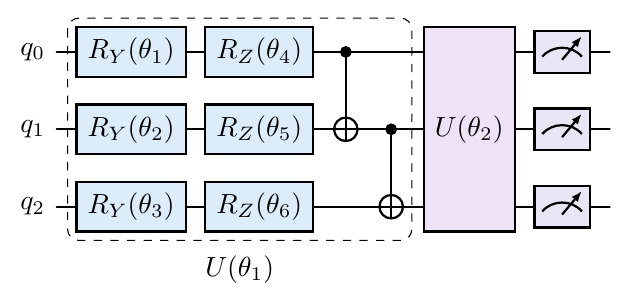
A three-qubit Born machine generates bitstrings by measuring a two-layer
AngleAnsatz. This example builds its sampling circuit and saves the complete
paper-ready LaTeX document; no training is needed to draw the topology.
from pathlib import Path
from qasp import create_qcbm, draw_qcbm

model = create_qcbm({
    "ansatz": "AngleAnsatz",
    "ansatz_config": {
        "n_layers": 2,
        "rotations": "YZ",
        "include_imprimitive": True,
        "imprimitive": "CNOT",
        "imprimitive_pattern": "chain",
    },
    "device": "default.qubit",
    "seed": 7,
}, n_qubits=3)
tex = draw_qcbm(model, output="tikz", tikz_options={
    "standalone": True, "symbolic_parameters": True, "compress": True,
})
Path("born_machine.tex").write_text(tex, encoding="utf-8")
Kernels
QFKernelFidelityKernelProjectedKernelcreate_kernel,draw_kernelKernelTargetAlignment,align_kernel,target_alignment
Quantum classification
PQCClassifier,QuantumClassifiercreate_classifier,draw_classifierClassifierTrainer,ClassifierLossClassProbabilityDecodermean_squared_error,hinge_lossbinary_cross_entropy,categorical_cross_entropyclassification_metrics,confusion_matrix,accuracy_score,f1_scoreroc_auc_score,pr_auc_score,average_precision_score
Combinatorial optimization
QUBOQAOA,WarmStartQAOARecursiveQAOA,RQAOALRQAOA,LinearRampQAOAPauliCorrelationEncoding,PCEcreate_optimizerdraw_optimization,draw_qaoa,draw_pce,draw_recursive_qaoa
from qasp import QAOA, QUBO

problem = QUBO.maxcut(3, [(0, 1), (1, 2), (0, 2)])
mixer = {
    "rotations": ["X 0", "X 1", "X 2", "XX 0 1"],
    "initial_state": "plus",
}

solver = QAOA(
    problem,
    n_layers=2,
    parametrization="multi_angle",
    mixer=mixer,
)
result = solver.solve(optimizer="COBYLA", optimizer_options={"maxiter": 100})
print(result.bitstring, result.energy)
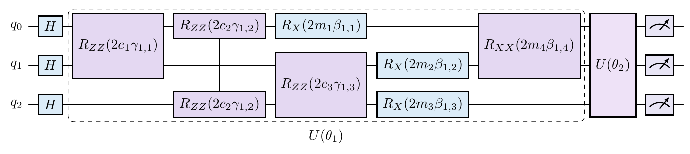
Draw the same two-layer, multi-angle QAOA circuit, including its custom
single-qubit X and two-qubit XX mixer. Symbolic labels show the parameter
structure independently of training. To show fitted numerical values instead,
pass parameters=result.parameters and set symbolic_parameters=False.
from pathlib import Path
from qasp import draw_optimization

tex = draw_optimization(
    solver, parameters=solver.initial_parameters("zeros"), output="tikz",
    tikz_options={"standalone": True, "symbolic_parameters": True, "compress": True},
)
Path("qaoa.tex").write_text(tex, encoding="utf-8")
Warm starts accept either a relaxed solution vector or True to compute a
bounded continuous relaxation. PCE accepts the same ansatz / ansatz_config
dictionary convention used by the classifier and RL factories. See
examples/optimization_algorithms.ipynb for executable examples of every
algorithm.
QAOA minimizes the expectation value of the QUBO Hamiltonian directly. With
analytic execution (shots=None), the default differentiation method is
adjoint. With finite-shot training, it switches to parameter-shift; either use
that gradient with a gradient-aware optimizer or train the noisy expectation
directly with a derivative-free optimizer such as COBYLA.
# Analytic Hamiltonian training with adjoint gradients.
analytic = QAOA(problem, n_layers=2)
analytic_result = analytic.solve(optimizer="BFGS", use_gradients=True)

# Finite-shot training followed by an independent 2,000-shot solution estimate.
sampled = QAOA(problem, n_layers=2, shots=500)
sampled_result = sampled.solve(
    optimizer="COBYLA",
    result_shots=2_000,
)
print(sampled_result.counts)
print(sampled_result.bitstring, sampled_result.solution_probability)

# Resample trained parameters at any later shot count.
counts = sampled.solution_counts(sampled_result.parameters, shots=10_000)
QAOA and PCE can train with either the default NumPy/Autograd backend or a
PyTorch backend. The NumPy backend supports the existing SciPy methods plus
PennyLane-native optimizers; the Torch backend uses torch.optim and keeps the
QNode, loss, gradients, and parameters as Torch tensors during training.
# PyTorch + adjoint differentiation on an analytic simulator.
torch_solver = QAOA(problem, n_layers=2, backend="torch")
torch_result = torch_solver.solve(
    optimizer="Adam",
    optimizer_options={"max_steps": 100, "lr": 0.05},
)

# PyTorch + parameter-shift differentiation with finite-shot training.
noisy_torch = QAOA(problem, backend="torch", shots=1_000)
noisy_result = noisy_torch.solve(
    optimizer="RMSprop",
    optimizer_options={"max_steps": 50, "lr": 0.02},
    result_shots=5_000,
)

# PennyLane optimizers use the NumPy/Autograd backend.
qng_result = QAOA(problem, backend="numpy").solve(
    optimizer="QNG",
    optimizer_options={"max_steps": 50, "stepsize": 0.02, "lam": 1e-3},
)
spsa_result = QAOA(problem, shots=1_000).solve(
    optimizer="SPSA",
    optimizer_options={"max_steps": 100, "a": 0.05, "c": 0.1},
)
Available optimizer families are exported as SCIPY_OPTIMIZERS,
PENNYLANE_OPTIMIZERS, and TORCH_OPTIMIZERS:
- SciPy: COBYLA, Nelder-Mead, Powell, BFGS, L-BFGS-B, and SLSQP.
- PennyLane: gradient descent, Adam, Adagrad, Momentum, Nesterov Momentum, RMSProp, quantum natural gradient (QNG), SPSA, quantum-natural SPSA (QNSPSA), and Shot Adaptive optimization.
- PyTorch: Adam, AdamW, SGD, RMSprop, Adagrad, Adadelta, ASGD, and LBFGS.
QNG, QNSPSA, and ShotAdaptive require a single scalar quantum objective,
so they apply directly to QAOA. PCE's loss is a nonlinear classical function
of several Pauli expectations; it supports the ordinary PennyLane gradient
optimizers and every listed Torch optimizer, but not those three QNode-only
optimizers. ShotAdaptive additionally requires finite-shot QAOA execution.
Optimization circuits use the same drawing outputs as the rest of QASP. TikZ exports default to symbolic QAOA parameters and can produce a complete, standalone paper-ready document:
tikz = sampled.draw(
    sampled_result,
    output="tikz",
    tikz_options={
        "standalone": True,
        "compress": True,
        "wire_labels": [r"q_0", r"q_1", r"q_2"],
        "gate_colors": {
            "single": "DCECF8",
            "two": "E4D8F2",
            "measurement": "E8E5F5",
        },
    },
)

# The high-level helper also constructs and draws a model from configuration.
tikz = draw_optimization(
    problem=problem,
    algorithm="multi_angle_qaoa",
    config={"n_layers": 2},
    output="tikz",
)
Use output="matplotlib" for a figure/axes pair or output="text" for an
ASCII circuit. PCE exposes the same .draw(...) method. After RQAOA.solve(),
rqaoa.draw(step=0, ...) draws any constituent recursive QAOA step.
Quantum-classifier examples
The classifier factory uses the same class-and-config notation as QASP's other modules. Probability readout returns a normalized distribution over any discrete number of classes; expectation readout returns one binary score or one score per class.
The two readout families have different mathematical meanings:
- Probability readout measures computational-basis Born probabilities and sums them into class probabilities with a contiguous, parity, or majority decoder. These outputs are genuine normalized quantum measurement probabilities and naturally pair with binary or categorical cross entropy.
- Expectation readout measures user-selected observables. For binary
classification QASP uses
score = mean(<O_1>, ..., <O_M>), predicts class 1 exactly whenscore > 0, and encodes MSE/hinge targets as{-1, +1}. The sigmoid values returned bypredict_probaare classical score post-processing, not Born probabilities. Multiclass expectation readout accepts either one observable per class or one nonempty observable group per class. It averages each group into its class score, applies temperature-softmax inpredict_proba, and predicts withargmax.
import torch
from qasp import ClassifierTrainer, create_classifier, draw_classifier

config = {
    "feature_map": "AngleEmbedding",
    "feature_map_config": {"rotations": "Y", "input_scaling": True},
    "ansatz": "AngleAnsatz",
    "ansatz_config": {
        "n_layers": 2,
        "rotations": "ZY",
        "include_imprimitive": True,
        "imprimitive_pattern": "ring",
        "reuploading": True,
    },
    "readout": "probabilities",
    "decoder": "parity",       # contiguous, parity, or majority
    "init": "small_normal",
}

classifier = create_classifier(config, n_qubits=4, n_classes=3)
trainer = ClassifierTrainer(
    classifier,
    objective="categorical_cross_entropy",
    learning_rate=0.02,
)
trainer.fit(
    torch.tensor(X_train, dtype=torch.float32),
    torch.tensor(y_train),
    epochs=20,
    batch_size=16,
    validation_data=(X_test, y_test),
)
metrics = trainer.evaluate(X_test, y_test)
# Includes metrics["roc_auc"] and metrics["pr_auc"]. PR AUC is step-wise
# average precision, which is usually more informative for rare positives.
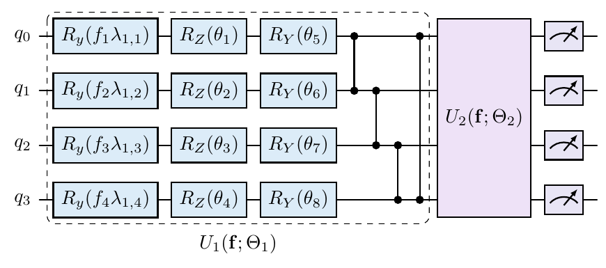
Export this classifier's Born-probability circuit with symbolic input scaling and a compact second reuploading layer. The parity class decoder is classical post-processing and is not drawn as a quantum gate.
from pathlib import Path

tex = draw_classifier(
    classifier, inputs=torch.zeros(4), output="tikz",
    tikz_options={"standalone": True, "symbolic_parameters": True, "compress": True},
)
Path("classifier_born.tex").write_text(tex, encoding="utf-8")
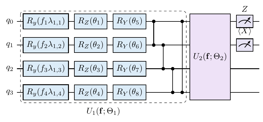
Binary expectation-value classification with an averaged custom observable and MSE is configured directly in the same notation:
expectation_config = {
    **config,
    "readout": "expectation",
    "decoder": None,
    "observable": ["Z 0", "ZZ 0 1", "X 1"],
}
classifier = create_classifier(expectation_config, n_qubits=4, n_classes=2)
trainer = ClassifierTrainer(classifier, objective="mean_squared_error")

# Publication-ready standalone Quantikz source with symbolic parameters.
tex = draw_classifier(
    classifier,
    inputs=torch.zeros(4),
    output="tikz",
    tikz_options={"standalone": True, "symbolic_parameters": True, "compress": True},
)
Path("classifier_expectation.tex").write_text(tex, encoding="utf-8")
For a three-class expectation classifier, nested groups define the observables whose expectation values are averaged into each class score:
multiclass_config = {
    **config,
    "readout": "expectation",
    "decoder": None,
    "observables": [
        ["Z 0", "X 0", "ZZ 0 1"],  # class 0
        ["Z 1", "X 1"],             # class 1
        ["Z 2", "X 2", "ZZ 2 3"],  # class 2
    ],
    "temperature": 0.8,
}
classifier = create_classifier(multiclass_config, n_qubits=4, n_classes=3)
scores = classifier(X_train[:8])
probabilities = classifier.predict_proba(X_train[:8])
Expectation and Born-probability classifiers can use the shared differentiable Pauli simulator. This example trains the expectation classifier with exact propagation:
pp_config = {
    **multiclass_config,
    "device": "PauliPropagationSimulator",
    "device_kwargs": {"k": None, "prune": False},
    "diff_method": "backprop",
    "shots": None,
}
classifier = create_classifier(pp_config, n_qubits=4, n_classes=3)
trainer = ClassifierTrainer(
    classifier,
    objective="categorical_cross_entropy",
    learning_rate=0.02,
)
trainer.fit(X_train, y_train, epochs=20, batch_size=16)
For Born readout, use readout="probabilities" with the same device fields
and the desired probability decoder. Dense probability reconstruction has the
readout limit described above. Optional approximations belong in
device_kwargs, for example {"k": 3, "prune": True, "topM": 20_000, "tau": 1e-10, "prune_every": 5}. Truncated values and gradients should be
checked against a feasible exact reference; prefer exact defaults for probability
losses. The legacy expectation-only lightning.pp adapters and their pp_*
arguments remain supported; see the migration guide.
For majority decoding, every majority block produces one code bit (strict
majority; even-block ties map to zero), blocks are interpreted most-significant
first, and the resulting integer is reduced modulo n_classes. Default blocks
are odd and maximize qubit coverage. Non-power-of-two class counts and explicit
even blocks can induce a non-uniform reference class prior; inspect
classifier.probability_decoder.reference_class_prior, or use
strict_majority_blocks=True to require equal, disjoint odd blocks of size at
least three with no unused measured wires.
For executable, assertion-driven sklearn integrations using Breast Cancer,
Iris, Wine, and Digits, see
examples/quantum_classifiers_sklearn_validation.ipynb.
For cross-module validation of cost and circuit-expectation concentration on classifiers, trainable kernels, and RL policies, see upstream examples/barren_plateau_diagnoser_validation.ipynb.
IQP quantum-kernel example
An IQP ansatz turns a kernel into a trainable QASP model while preserving the same feature-map, device, and differentiation configuration used elsewhere in the package:
from qasp import create_kernel

config = {
    "kernel_type": "fidelity",  # or projected
    "feature_map": "AngleEmbedding",
    "feature_map_config": {
        "rotations": "Y",
        "imprimitive_pattern": "ring",
    },
    "ansatz": "IQPAnsatz",
    "ansatz_config": {
        "n_layers": 2,
        "imprimitive_pattern": "ring",
        "reuploading": True,
    },
    "device": "default.qubit",
}

kernel = create_kernel(config, n_qubits=4)
K_train = kernel.gram(X_train)
K_test = kernel.gram(X_test, X_train)

# Localized fidelity uses the same class with explicit projector subsets.
local_config = {
    **config,
    "projectors": ["P 0 1", "P 0 2", "P 0 1 2"],
}
local_kernel = create_kernel(local_config, n_qubits=4)
The fidelity circuit evaluates an overlap between the two encoded samples.
This example keeps every gate visible because mirrored layer compression
requires reuploading=False. Open the vector PDF to inspect the full-width
circuit. QASP labels the forward input as x and the adjoint input as y.
Both halves reuse the same variational angles and input scales.
from pathlib import Path
import numpy as np
from qasp import draw_kernel

tex = draw_kernel(
    kernel=kernel, x=np.zeros(4), y=np.ones(4), output="tikz",
    tikz_options={
        "standalone": True,
        "symbolic_parameters": True,
    },
)
Path("fidelity_kernel.tex").write_text(tex, encoding="utf-8")

With no projectors key, FidelityKernel measures the global all-zero
projector. Each explicit projector label "P i j ..." measures the probability that the listed
qubits are jointly in the all-zero state, with the identity on every unlisted
qubit. A single projector containing every qubit recovers global fidelity.
For proper subsets, this localized similarity is not guaranteed to be PSD for
arbitrary encoding circuits; inspect the Gram spectrum before using it with a
method that assumes a Mercer kernel.
See examples/iqp_quantum_kernels.py for global and localized modes of
FidelityKernel, projected features, and trainable kernel-target alignment.
For an assertion-driven notebook covering circuit drawings, Gram diagnostics,
gradients, and precomputed-kernel SVMs for every kernel class, run
examples/iqp_quantum_kernels_validation.ipynb.
RL / training / analysis
create_modeldraw_modelPQCBornPQCSoftmaxPQCBornVarianceLearnablePQCBornFastTruncatedPauliPropREINFORCETorchRLTrainerContextualBanditTrainerpolicy_variancecompute_DLA_generatorsfourier_analysishadamard_decompositioncz_decompositioncnot_decomposition
Distributed statevector simulation (MPI)
Pass device="lightning.kokkos", mpi=True to QAOA (including warm-start and
linear-ramp variants), PCE, RQAOA, classifiers, kernels, RL policies, or
CircuitBuilder.compile. Classifier and RL configurations also retain the
older enable_mpi=True alias where it was previously supported. Kernels
already accepted mpi; all named device paths now forward it, including
lightning.gpu and custom MPI-capable plugins. Unsupported plugins raise
their own error; QASP does not fall back to a serial device.
from qasp import QAOA, QUBO, PCE, RecursiveQAOA, create_classifier, create_kernel

problem = QUBO.maxcut(30, [(i, i + 1) for i in range(29)])
solver = QAOA(
    problem, device="lightning.kokkos", mpi=True,
    backend="torch", diff_method="adjoint", seed=42,
    device_kwargs={"batch_obs": True},
)
result = solver.solve(
    optimizer="Adam", optimizer_options={"max_steps": 50, "lr": 0.02},
    result_shots=1000, include_probabilities=False,
)
# Counts-only results avoid allocating a 2**n probability vector on each rank.
print(result.bitstring, result.solution_probability)

# PCE also accepts device/mpi/device_kwargs inside its circuit dictionary.
pce = PCE(problem, device="lightning.kokkos", mpi=True, seed=42)
recursive = RecursiveQAOA(
    problem, device="lightning.kokkos", mpi=True, cutoff=10,
    qaoa_options={"seed": 42},
)
# Use result_shots=... and include_probabilities=False in recursive.solve()
# for counts-only step results and direct Z/ZZ correlation measurements.

# Add these options to existing classifier/kernel factory dictionaries:
distributed_options = {
    "device": "lightning.kokkos", "mpi": True, "diff_method": "adjoint",
}
# classifier = create_classifier({**classifier_config, **distributed_options}, n_qubits, n_classes)
# kernel = create_kernel({**kernel_config, **distributed_options}, n_qubits)
Launch the same script on every MPI rank using the cluster's MPI-enabled
PennyLane/Lightning installation. All ranks must execute the same circuit
calls in the same order, with identical parameters, data, optimizer state,
and minibatches. Seed NumPy and Torch identically before model construction;
pass the same explicit seed to QAOA/PCE and stochastic optimizers. Only
printing and file writes should be restricted to rank zero. Do not scatter
different kernel pairs or training examples across ranks sharing one
distributed statevector. QASP forwards the device configuration; it does not
synchronize a user's classical training loop or replace it with distributed
data-parallel training.
Use adjoint differentiation for supported analytic expectation measurements,
and parameter-shift for finite shots. Classifiers and RL policies default to diff_method="best"
so PennyLane can select a method supported by the device. An explicitly chosen
backprop method is not supported by Lightning. Measurements, observables,
and gradient transforms must be supported by the installed plugin version.
Full-state outputs, full probability readouts, PQCBM NLL, and QFKernel
can still require exponential host memory; MPI distributes the
simulator state, not those classical arrays. Prefer expectation readouts or
small measurement registers for classifiers. PQCBM MMD trains directly on
Pauli-Z expectations without constructing the full probability vector. include_probabilities=False
requires result_shots and returns probabilities=None, with sparse counts
and solution_probability retained. The default result format is unchanged.
Keep enough qubits per MPI rank in compressed PCE registers and at the RQAOA
cutoff; RQAOA does not shrink the MPI communicator as variables are eliminated.
Additional device constructor options are accepted via device_kwargs in
optimization, classifiers, kernels, PQCBM, and the circuit builder.
For an already constructed PennyLane device/QNode, enable MPI at creation;
QASP reuses it and cannot turn a serial object into an MPI object.
PauliPropagationSimulator and the legacy lightning.pp adapters do not
support MPI and reject mpi=True.
Cluster validation (small deterministic circuits, serial-reference comparisons, gradients, a QAOA optimizer step, and sampled results):
mpiexec -n 2 python tests/tests_deucalion/mpi_modules_smoke.py --device lightning.kokkos --qubits 6
Use your scheduler's equivalent launcher, such as srun, when required.
The plugin must be compiled with MPI support; see the official
Lightning-Kokkos MPI documentation.
Manual circuit construction example
QASP can also be used without the policy classes. You can directly combine a feature map, an ansatz template, and CircuitBuilder to create a differentiable torch-compatible quantum layer.
The example below follows the same style used in upstream tests/test_qml_models.ipynb.
from qasp import AngleEmbedding, AngleAnsatz, CircuitBuilder
import pennylane as qml
from pennylane import numpy as np
import torch

# 1. Define a feature map
fm = AngleEmbedding(
    features=4,
    n_qubits=4,
    rotations="YZ",
    input_scaling=True,
)

# 2. Define an ansatz that reuses the feature map
ansatz = AngleAnsatz(
    n_qubits=4,
    n_layers=3,
    rotations="ZY",
    feature_map=fm,
    include_imprimitive=True,
    imprimitive="CZ",
    imprimitive_pattern="all_to_all",
    reuploading=True,
)

# 3. Inspect required parameter shapes
shapes = ansatz.get_param_shapes()
print("Parameter shapes:", shapes)

# Example initialization
input_scaling_params = np.random.uniform(-1.0, 1.0, size=shapes[0])
params = np.random.uniform(-np.pi, np.pi, size=shapes[1])

# 4. Build a circuit with an expectation-value readout
builder = CircuitBuilder(n_qubits=4)
builder.set_ansatz(ansatz)
builder.set_measurement(
    "expectation",
    wires=[0, 1, 2, 3],
    observables=["Z 0", "Z 1", "ZZ 0 1", "ZZ 2 3"],
)

circuit = builder.build()
qnode = builder.compile(device="lightning.qubit", diff_method="adjoint")

# 5. Create a torch layer
qlayer = builder.create_torchlayer(
    params=torch.tensor(params, requires_grad=True),
    input_scaling_params=torch.tensor(input_scaling_params, requires_grad=True),
)

# 6. Evaluate the layer on sample input
x = torch.tensor([0.1, -0.2, 0.3, 0.5], dtype=torch.float32)
out = qlayer(x)
print("Quantum layer output:", out)
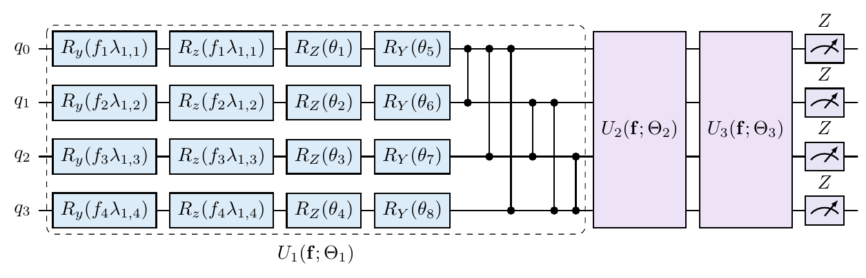
Export this same builder, passing its input and both parameter arrays. The first layer includes the feature map; subsequent blocks include reuploading and are labelled as data-dependent unitaries.
state = qlayer.state_dict()
builder.save_tikz(
    "manual_circuit.tex",
    inputs=x, params=state["params"],
    input_scaling_params=state["input_scaling_params"],
    standalone=True, symbolic_parameters=True, compress=True,
)
This lower-level workflow is useful when:
- designing a custom model architecture,
- testing a new feature map or ansatz,
- studying trainability or Fourier structure without committing to a specific RL algorithm,
- integrating a QASP circuit into a larger PyTorch model.
High level RL policies from dictionaries and create_model
This is the main high-level workflow for reinforcement learning with QASP.
from qasp import create_model, draw_model
import torch

n_qubits = 6

fm_config = {
    "features": 4,
    "rotations": "Z",
}

ansatz_config = {
    "n_layers": 3,
    "rotations": "ZY",
    "reuploading": False,
    "include_imprimitive": True,
    "imprimitive": "CZ",
    "imprimitive_pattern": "all_to_all",
    "include_final_imprimitive": False,
    "include_feature_map_first": False,
    "include_hadamards_initial": True,
}

observables = [f"Z {i}" for i in range(n_qubits)]
observables += [f"ZZ {i} {i+1}" for i in range(n_qubits - 1)]

policy_model_config = {
    "ansatz": "AngleAnsatz",
    "ansatz_config": ansatz_config,
    "feature_map": "NeuralEmbedding",
    "feature_map_config": fm_config,
    "n_actions": 2,
    "init": "normal_0_1",
    "device": "lightning.qubit",
    "diff_method": "adjoint",
    "fc_layer": True,
    "observables": observables,
}

policy = create_model("PQCSoftmax", policy_model_config, n_qubits=n_qubits)
To visualize the resulting circuit:
draw_model(
    model=policy,
    policy_class="PQCSoftmax",
    n_qubits=n_qubits,
    num_inputs=4,
    inputs=torch.zeros(4),
)
Save a paper-ready figure of this six-qubit neural-embedding policy. This configuration places its feature map after the first variational layer, so the export shows all three layers without automatic compression. The classical neural feature map and final affine policy head are not quantum gates. Open the vector PDF to inspect the individual gates at full size.
from pathlib import Path

tikz = draw_model(
    model=policy, inputs=torch.zeros(4), output="tikz",
    tikz_options={"standalone": True, "symbolic_parameters": True},
)
Path("neural_policy.tex").write_text(tikz, encoding="utf-8")

Exporting publication-ready TikZ circuits
QASP can export any CircuitBuilder, PennyLane QNode, quantum function, or
quantum tape as editable vector-quality LaTeX using the quantikz package:
from qasp import circuit_to_tikz, save_tikz

# `params` and `inputs` are the same values used to execute the circuit.
tikz = circuit_to_tikz(
    policy.circuit,
    inputs=torch.zeros(4),
    params=policy.qlayer.state_dict()["params"],
    symbolic_parameters=True,
)
print(tikz)

# A complete, directly compilable .tex document:
save_tikz(
    "policy_circuit.tex",
    policy.circuit,
    inputs=torch.zeros(4),
    params=policy.qlayer.state_dict()["params"],
    standalone=True,
)
For a builder, the same operations are also available as methods:
tikz = builder.to_tikz(params=params, symbolic_parameters=True)
builder.save_tikz("circuit.tex", params=params, standalone=True)
By default, the result is a snippet ready to paste into a paper or Beamer
presentation (add \\usepackage{xcolor} and \\usepackage{quantikz} to the preamble). Set
standalone=True for a complete document. Use wire_labels,
parameter_labels, or parameter_formatter to match the notation of a paper.
An AngleEmbedding block is expanded into its individual rotations. With
symbolic parameters, encoded angles are labelled f_i, or
f_i\\lambda_i when input scaling is enabled; variational angles retain
the independent \\theta_i sequence.
The default pastel theme uses light blue for single-qubit gates, purple for
two-qubit gates, pale violet for larger gates, and lavender for measurements.
Override any color with an HTML hex value or an existing xcolor expression:
tikz = builder.to_tikz(
    params=params,
    gate_colors={
        "single": "DCECF8",
        "two": "E4D8F2",
        "multi": "violet!10",
        "measurement": "blue!8",
    },
)
Set gate_colors=False to generate an unfilled monochrome circuit.
For deep repeated circuits, set compress=True. QASP keeps the data-encoding
prefix visible, draws every gate in the first variational layer inside a dashed
U(\\theta_1) enclosure, and replaces later layers with register-wide unitary
blocks:
tikz = draw_model(
    model=policy,
    inputs=torch.zeros(4),
    output="tikz",
    tikz_options={
        "standalone": True,
        "symbolic_parameters": True,
        "compress": True,
        "max_explicit_layers": 4,
    },
)
For n_layers <= max_explicit_layers, every later block from
U(\\theta_2) through U(\\theta_L) is displayed. Larger circuits show
U(\\theta_2), an ellipsis, and U(\\theta_L). Layer boundaries are inferred
automatically for AngleAnsatz and IQPAnsatz. With data reuploading, each
compressed block includes its feature map and is labelled as data-dependent;
the encoding must precede the first layer. Input-scaling symbols include the
layer index. Mirrored overlap compression still requires reuploading=False.
The same exporter is available through draw_kernel. Fidelity and local
fidelity kernels use both samples; projected kernels only need x:
from qasp import draw_kernel

tikz = draw_kernel(
    kernel=kernel,
    x=X_train[0],
    y=X_train[1],  # omit for a projected kernel
    output="tikz",
    tikz_options={
        "standalone": True,
        "symbolic_parameters": True,
        "compress": False,  # show both uploads and their shared weights
    },
)
Compression applies to trainable kernels built with a repeated
AngleAnsatz or IQPAnsatz and reuploading=False. Feature-map-only
kernels can still be exported to TikZ, but have no variational layers to
compress. For fidelity and local-fidelity circuits, QASP also draws the
matching adjoint blocks in reverse order, from
U^\\dagger(\\theta_L) through U^\\dagger(\\theta_1).
For runnable drawing-only examples covering IQP and AngleAnsatz policies, fidelity, local-fidelity, and projected kernels, and a directly assembled CircuitBuilder, see the circuit-drawing notebook. Each module example above and the CartPole examples below include their own drawing, editable LaTeX, and vector PDF. Export calls can run immediately after model construction; training is not required. Symbols describe the circuit structure rather than a fitted parameter value. Readout meters are schematic: tensor-product observables use local basis meters, and overlapping observables share wires. The observable lists in the code specify the complete set of expectations, including correlations and measurements in different bases.
QASP returns LaTeX source. With a TeX distribution containing standalone,
xcolor, and quantikz, compile any saved figure (replace the filename with
the one from your example):
pdflatex -interaction=nonstopmode -halt-on-error born_machine.tex
For inclusion in an existing paper, set standalone=False and add
\usepackage{xcolor} and \usepackage{quantikz} to its preamble, or use
\includegraphics{born_machine.pdf} with the graphicx package.
To regenerate every README figure from the marked construction/export code blocks, without running the training examples:
python examples/render_readme_circuits.py
This uses QASP's installed dependencies, pdflatex, and Poppler's pdftoppm.
The editable sources, vector PDFs, and PNG previews are written to
docs/assets/circuits/. Use --source-only to export
LaTeX without a TeX installation. The generator executes only the blocks
marked readme-circuit in this README; blocks sharing a name share variables.
Reinforcement learning example with REINFORCE
QASP includes a built-in REINFORCE trainer for policy-gradient experiments.
CartPole with a softmax PQC policy
from qasp import *

agent = REINFORCE(
    policy=policy,
    env_name="CartPole-v1",
    gamma=0.99,
    lr=1e-2,
    batch_episodes=16,
    logits=True,  # PQCSoftmax.forward returns action logits.
    normalize_mode="clip",
    baseline_type="ema",
    normalize_returns=True,
    entropy_coef=0.01,
    max_grad_norm=1.0,
    fc_layer=True,
)

returns = agent.train(num_episodes=500)
Typical REINFORCE controls
The trainer supports several knobs that are useful in experiments:
baseline_type="ema"orbaseline_type="value"normalize_modefor state preprocessingentropy_coeffor exploration pressurebatch_episodesfor lower-variance policy-gradient updatesmax_grad_normfor gradient clippingfc_layer=Truefor policies that use a classical readout head on top of quantum expectations
This makes it straightforward to compare PQC policies across environments such as CartPole, Acrobot, and contextual bandits.
Policy classes in qasp.rl.policies
QASP currently exposes several policy-model families.
PQCBorn
The direct class is a legacy sampler whose forward returns an action and log
probability. The factory selector create_model("PQCBorn", ...) instead constructs
PQCBornVariance, the current probability-returning decoder model.
PQCSoftmax
An expectation-score model with an optional biased affine head. forward()
returns logits; use a logits-aware trainer or Categorical(logits=...). The legacy
action_probs() shortcut bypasses the head and PP path. fc_layer=None disables
the head; any non-None value currently creates one.
PQCBornVariance
The current Born-policy implementation, with contiguous, prefix-parity, hidden and majority-modulo decoders. It supports compatible probability, expectation reconstruction and majority sparse-projector paths; backend restrictions are documented on the constructor.
LearnablePQCBorn
A historical adaptive-measurement prototype. Its setup and postprocessing have known limitations; it is not a validated replacement for the fixed-decoder APIs.
Trainability and analysis utilities
The lazy top-level barren_plateau_diagnoser works with a constructed QASP
classifier, trainable kernel, or RL policy. It repeatedly samples the selected
trainable parameters and reports both the unbiased finite-sample variance of
one scalar cost and the variance of every raw quantum expectation output,
together with their running variance after every sample:
import torch
from qasp import barren_plateau_diagnoser, target_alignment

diagnosis = barren_plateau_diagnoser(
    classifier,
    n_samples=2000,
    initialization="random_-pi_pi",
    state=torch.tensor(X_train[0]),  # fixed input: variance over parameters
    targets=torch.tensor(y_train[0]),
    objective="mean_squared_error",
    seed=7,
    return_samples=True,
)

print(diagnosis["variance"])
print(diagnosis["cost_variance"])
print(diagnosis["expectation_value_variance"])
print(diagnosis["expectation_variance"])
cost_variance_curve = diagnosis["cost_variance_by_sample"]
expectation_variance_curve = diagnosis["expectation_value_variance_by_sample"]
The actual system-size scaling experiment uses a model factory and a qubit
list. Each width receives its own independent ensemble of n_samples
initializations:
qubit_list = [2, 4, 6, 8, 10, 12, 14, 16]

diagnosis = barren_plateau_diagnoser(
    model_factory=lambda n: create_classifier(classifier_config(n), n, 2),
    qubit_list=qubit_list,
    n_samples=2000,
    initialization="random_-pi_pi",
    state_factory=lambda n: torch.zeros(n),  # fixed input at each width
    seed=7,
)

# Arrays aligned one-to-one with qubit_list.
cost_variance_vs_qubits = diagnosis["cost_variance"]
expectation_variance_vs_qubits = diagnosis["expectation_value_variance"]
per_width_details = diagnosis["results_by_qubit"]
Here classifier_config(n) denotes a user factory for the same circuit family
at width n. The sweep also accepts kernel and policy factories. Raw-output
dimensionality can change with width, so componentwise values are stored as
expectation_variance_by_qubit[n]; scalar cost and mean-expectation variances
are returned as arrays that can be plotted directly against qubit_list on a
logarithmic variance axis.
variance remains a compatibility alias for cost_variance. Observable
circuits report the variance of each measured expectation before decoder,
scaling, softmax, or loss post-processing. For Born/probability circuits, QASP
uses the raw basis probabilities to reconstruct one local Pauli-Z expectation
per measured qubit. expectation_value_variance is the scalar variance of the
arithmetic mean of those raw outputs and therefore includes their covariance;
expectation_variance retains the componentwise variances.
expectation_function(model, sampled_state) can override this default when a
custom quantum statistic is required. With return_samples=True, the
corresponding raw values are available as cost_samples,
expectation_value_samples, and expectation_samples.
When targets are omitted, the classifier default is the class probability
at output_index; the policy default is the action probability at that index;
and the kernel default is k(x, y) for a supplied pair state=(x, y). For an
actual task objective, pass cost_function(model, sampled_state). For example,
a trainable kernel can diagnose negative target alignment on a fixed dataset:
diagnosis = barren_plateau_diagnoser(
    kernel,
    n_samples=500,
    state=X_train,
    cost_function=lambda model, X: -target_alignment(model.gram(X), y_train),
    initialization="small_normal",
    seed=11,
)
If state=None, QASP samples a fresh embedded input per initialization with
state_initialization (a pair for kernels). This estimates joint variance over
parameters and inputs. Supplying state instead isolates parameter variance
conditional on that fixed input. state_sampler supports custom per-sample
data generation, and parameter_scope="all" includes trainable classical
post-processing parameters rather than only the quantum qlayer. The original
model parameters and train/evaluation mode are restored even if a sample
fails.
These are initialization variances of the cost and of expectation values—not
the within-circuit quantum measurement variance
<O^2> - <O>^2. They are useful concentration signals, but the standard
barren-plateau claim concerns how gradient variance scales with system size;
a controlled cost-variance sweep alone does not establish that stronger
claim without a corresponding gradient analysis.
The legacy qasp.rl.metrics module provides probability-variance sampling and
heuristic Lie-closure utilities. compute_DLA_generators returns closure sizes;
the named gate-decomposition helpers supply heuristic generator lists rather
than executable unitary decompositions. fourier_analysis performs no Fourier
transform and has legacy import limitations. Use the package guide
to distinguish these prototypes from the current concentration diagnostics.
Notebooks and example scripts
See the curated example index for tutorials covering circuits, initialization, RL, classifiers, kernels, generative learning, optimization and both QASP simulators. Notebooks are stored without outputs. The cluster scripts cover distributed execution.
Historical experiment notebooks, stored datasets and papers are linked from the repository layout guide rather than included in this checkout.
Quantum deep Q-learning
qasp.rl.qfunctions provides PQDQN and create_qfunction for dictionary-driven
quantum action-value networks, with shared or per-action Pauli strings and exact
parity/majority-modulo Pauli features with configurable preset_actions.
The fully connected layer includes a bias for presets and shared observables;
n_actions independently controls the final number of Q-values.
PQDQN supports device="PauliPropagationSimulator",
device_kwargs={"k": None, "prune": False}, and diff_method="backprop"
for exact differentiable Pauli propagation with the same DeepQLearning trainer.
Use batch_mode="sequential" with neural embeddings. Optional truncation and
pruning belong in device_kwargs; the legacy device="lightning.pp" route
and its pp_* arguments remain available for existing experiments.
qasp.rl.torchrl.DeepQLearning adds replay-based DQN/Double DQN with a frozen
target network and epsilon-greedy exploration.
draw_qfunction(model, output="tikz", tikz_options=...) and model.draw(...)
use the same Quantikz exporter as policies and kernels, including full/compact
views, symbolic parameters, pastel colors, and standalone or paper snippets.
The example notebooks compile vector PDFs and display PDF-rendered previews.
See the Q-function guide, observable validation notebook, the CartPole training notebook, and the 10-qubit PP/Lightning benchmark. The benchmark records inference and gradient timings alongside truncation errors. Runtime improvements should be assessed separately from approximation quality and reinforcement-learning performance.
End-to-end CartPole examples
Each example below runs independently after installing QASP and its dependencies.
Both use four qubits for CartPole's four observations, two actions, and the
default.qubit simulator. Six short episodes make these examples quick checks
of construction and training; they do not establish convergence. Increase the
training budget and episode cap for a learning experiment.
Policy gradients with softmax or Born policies
Choose PQCSoftmax to turn learned action logits into a categorical policy, or
PQCBorn to decode circuit probabilities into action probabilities. The
create_model("PQCBorn", ...) factory constructs the current
PQCBornVariance implementation. Set the trainer's logits flag to match the
selected model's output.
from qasp.rl import create_model, draw_model
from copy import deepcopy
import torch

torch.manual_seed(7)
policy_kind = "PQCSoftmax"  # Change to "PQCBorn" for a Born policy.
config = {
    "n_actions": 2,
    "ansatz": "AngleAnsatz",
    "ansatz_config": {
        "n_layers": 2,
        "rotations": "YZ",
        "reuploading": True,
        "include_imprimitive": True,
        "imprimitive": "CNOT",
        "imprimitive_pattern": "ring",
    },
    "feature_map": "AngleEmbedding",
    "feature_map_config": {
        "features": 4,
        "rotations": "Y",
        "input_scaling": True,
    },
    "device": "default.qubit",
    "diff_method": "backprop",
}
if policy_kind == "PQCSoftmax":
    config.update(observables=["Z 0", "Z 1", "Z 2", "Z 3"], fc_layer=True)
else:
    config.update(
        policy="parity-like",
        parity_cnot_decomposition=False,
        training_method="probs",
    )

# Copy nested dictionaries because the policy factory resolves them in place.
policy = create_model(policy_kind, deepcopy(config), n_qubits=4)
from qasp.rl import REINFORCE

with torch.no_grad():
    output = policy(torch.zeros(4))
    probabilities = output.softmax(dim=-1) if policy_kind == "PQCSoftmax" else output
    action = torch.distributions.Categorical(probs=probabilities).sample().item()
print("Initial action probabilities:", probabilities.tolist(), "sampled action:", action)

agent = REINFORCE(
    policy=policy,
    env_name="CartPole-v1",
    device="cpu",
    logits=(policy_kind == "PQCSoftmax"),
    normalize_mode="tanh",
    lr=0.01,
    batch_episodes=2,
    max_steps=50,
    baseline_type="ema",
)
try:
    agent.env.reset(seed=7)  # Seed subsequent environment resets as well.
    returns = agent.train(num_episodes=6, log_every=2)
finally:
    agent.env.close()
print("Training episode returns:", returns)
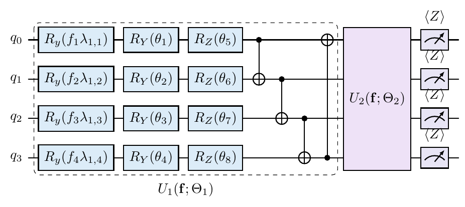
Save the paper-ready circuit for the selected policy. The drawing below
shows the default softmax policy's four Z readouts before the classical head.
from pathlib import Path

policy_tex = draw_model(
    model=policy, inputs=torch.zeros(4), output="tikz",
    tikz_options={"standalone": True, "symbolic_parameters": True, "compress": True},
)
Path("cartpole_policy.tex").write_text(policy_tex, encoding="utf-8")
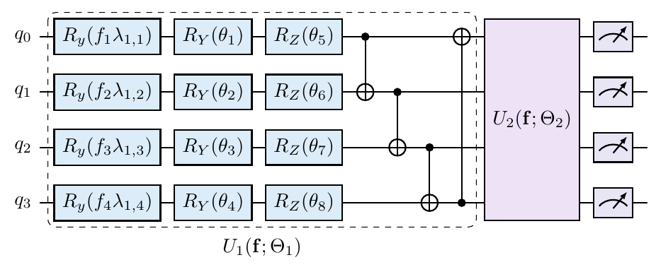
For comparison, build the Born-policy variant from the same ansatz and feature map. Its computational-basis measurements feed the classical parity decoder.
born_config = deepcopy(config)
born_config.pop("observables", None)
born_config.pop("fc_layer", None)
born_config.update(
    policy="parity-like", parity_cnot_decomposition=False, training_method="probs",
)
born_policy = create_model("PQCBorn", born_config, n_qubits=4)
born_tex = draw_model(
    model=born_policy, inputs=torch.zeros(4), output="tikz",
    tikz_options={"standalone": True, "symbolic_parameters": True, "compress": True},
)
Path("cartpole_born.tex").write_text(born_tex, encoding="utf-8")
REINFORCE.train() returns unshaped training-episode returns. Its
normalize_mode preprocesses observations before the policy call. The legacy
trainer freezes CartPole optimization when its trailing training mean reaches
195; use independent evaluation when assessing performance on CartPole-v1.
Q-learning with PQDQN
create_qfunction constructs a PQDQN. This example measures four Pauli-Z
features and learns an affine map to two Q-values. DeepQLearning trains with
replay minibatches, a separate target network, and epsilon-greedy exploration;
Double DQN is enabled explicitly below. Greedy evaluation uses a separate
environment and performs no training updates.
from qasp.rl import create_qfunction, draw_qfunction
import torch

torch.manual_seed(7)
config = {
    "ansatz": "AngleAnsatz",
    "ansatz_config": {
        "n_layers": 2,
        "rotations": "YZ",
        "reuploading": True,
        "include_imprimitive": True,
        "imprimitive": "CNOT",
        "imprimitive_pattern": "ring",
    },
    "feature_map": "AngleEmbedding",
    "feature_map_config": {
        "features": 4,
        "rotations": "Y",
        "input_scaling": True,
    },
    "observables": ["Z 0", "Z 1", "Z 2", "Z 3"],
    "fc_layer": True,
    "fc_bias": True,
    "input_activation": "tanh",
    "device": "default.qubit",
    "diff_method": "backprop",
    "batch_mode": "broadcast",
}
qfunction = create_qfunction(config, n_qubits=4, n_actions=2)
from qasp.rl import DeepQLearning

with DeepQLearning(
    qfunction,
    "CartPole-v1",
    lr=0.01,
    batch_size=8,
    learning_starts=16,
    train_frequency=4,
    target_update_interval=10,  # Measured in optimizer updates.
    double_dqn=True,
    epsilon_decay_steps=200,
    max_steps=50,
    seed=7,
) as trainer:
    history = trainer.train(num_episodes=6, log_every=2)
    evaluation_returns = trainer.evaluate(num_episodes=3, seed=10000)

print("Training episode returns:", [row["return"] for row in history])
print("Mean greedy evaluation return:", sum(evaluation_returns) / len(evaluation_returns))
with torch.no_grad():
    q_values = qfunction(torch.zeros(4))
print("Q-values:", q_values.tolist(), "greedy action:", q_values.argmax().item())
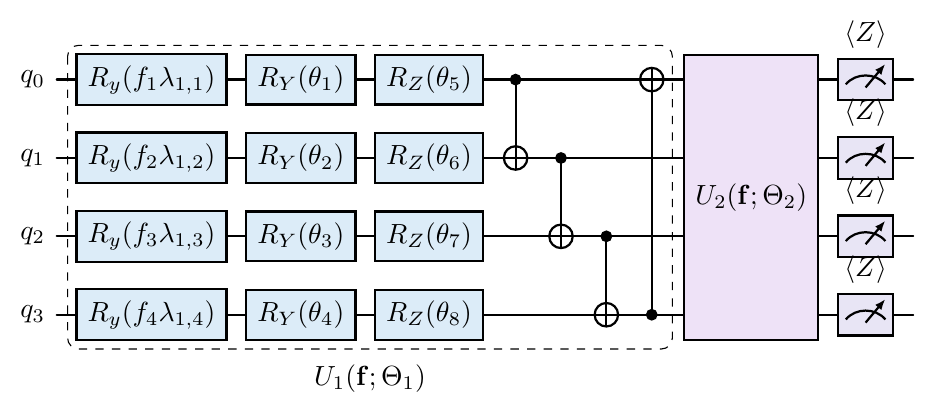
Export this PQDQN's quantum feature circuit; the learned affine map from four measured expectations to two Q-values is classical and is not drawn.
from pathlib import Path

qfunction_tex = draw_qfunction(
    qfunction, inputs=torch.zeros(4), output="tikz",
    tikz_options={"standalone": True, "symbolic_parameters": True, "compress": True},
)
Path("pqdqn.tex").write_text(qfunction_tex, encoding="utf-8")
The affine head produces unconstrained action values, so greedy action
selection uses argmax. To use a predefined readout, replace observables
with "parity-like" or "majority-modulo" and set preset_actions=2 in the
model dictionary. These presets supply Pauli features to the same learned head.
For longer experiments, saved results, and additional readout choices, see the CartPole PQDQN notebook, Q-function guide, and policy training notebook.
Citing QASP
If you use QASP in a paper or other research output, please cite the software. Citation metadata is provided in CITATION.cff, crediting INESC TEC.
1 maintainer

Metadata
1 maintainer
Release files for qasp 0.1.3
For a detailed explanation of source distributions (sdists) and built distributions (wheels), please see the package formats documentation.
Source distribution (sdist)
| File | Size | Uploaded | Provenance | Actions |
|---|---|---|---|---|
| qasp-0.1.3.tar.gz | 369.3 kB | With provenance | Details for qasp-0.1.3.tar.gz |
Built distribution (wheel)
| File | Interpreter | ABI | Platform | Actions Reset |
|---|---|---|---|---|
| qasp-0.1.3-py3-none-any.whl | Python 3 | none | any | Details for qasp-0.1.3-py3-none-any.whl |
Total release size: 653.2 kB
Release files / qasp-0.1.3.tar.gz
| Download URL | qasp-0.1.3.tar.gz |
|---|---|
| Size | 369.3 kB |
| Tags | Source |
|
SHA-256 checksum How to use checksums |
835ae9f01302f005d2f72c340d61c7f392feb57db56b77ff3147f19b1214b468
|
|
BLAKE2b-256 checksum How to use checksums |
9463a1861b766735da727d3e67bad47f79830d69d2cf1956fb6f6026b36521b6
|
| Upload date | |
|
Uploaded using Trusted Publishing? What is trusted publishing? |
Yes |
| Uploaded via |
twine/7.0.0 CPython/3.13.16
|
Provenance
Provenance describes where a file came from. On PyPI, provenance is shared via attestations, which provide a verifiable record of the build or publishing details. View details, limitations and caveats.


PyPI Publish Attestation
PyPI verified that this artifact, at this checksum, originated from the publisher listed below.
Signed by GitHub Actions, verified by PyPI on Nov 5, 2026.
Transparency logRelease files / qasp-0.1.3-py3-none-any.whl
| Download URL | qasp-0.1.3-py3-none-any.whl |
|---|---|
| Size | 283.9 kB |
| Tags | Python 3 |
|
SHA-256 checksum How to use checksums |
94fcfa2a43ba4c60e63dc881adc8f6899531903f9d38b50336c7a9b437df5e61
|
|
BLAKE2b-256 checksum How to use checksums |
47050d47d9890d2debd05f09c430cca389932455c68ddb7bc5f698c66eeaec79
|
| Upload date | |
|
Uploaded using Trusted Publishing? What is trusted publishing? |
Yes |
| Uploaded via |
twine/7.0.0 CPython/3.13.16
|
Provenance
Provenance describes where a file came from. On PyPI, provenance is shared via attestations, which provide a verifiable record of the build or publishing details. View details, limitations and caveats.
PyPI Publish Attestation
PyPI verified that this artifact, at this checksum, originated from the publisher listed below.
Signed by GitHub Actions, verified by PyPI on Nov 5, 2026.
Transparency logSecurity for qasp 0.1.3
Provenance
Provenance describes where a file came from. On PyPI, provenance is shared via attestations, which provide a verifiable record of the build or publishing details. View details, limitations and caveats.
Full provenance
All 2 files in this release have been uploaded with provenance metadata.
Attestation for qasp-0.1.3.tar.gz
PyPI Publish Attestation
PyPI verified that this artifact, at this checksum, originated from the publisher listed below.
Signed by GitHub Actions, verified by PyPI on Nov 5, 2026.
Transparency logA note on package security
PyPI is a repository for distributing packages, not a service for auditing them. While third-party security researchers and our staff do their best to detect and remove malicious packages, PyPI cannot guarantee the quality, security or suitability of any given package.
To learn more about protecting yourself from malicious actors, visit our package security documentation.















