Lattice QED Hamiltonian for Quantum Computing


Project description

Lattice QED Hamiltonian for Quantum Computing
This repository contains useful Python functions and classes for seamlessly designing and obtaining Quantum Electrodynamic (QED) Hamiltonians for 1D, 2D or 3D lattices with staggered fermionic degrees of freedom, i.e., Kogut and Susskind formulation[^1].
The implementation is useful for carrying out research on QED quantum simulation assisted by quantum computing and quantum algorithms, as well as for analysis and comparison with known exact-diagonalization (ED) methods. In turn, the classes in this module are compatible with exact diagonalization libraries and the Qiskit library.
Related work:
- Analysis of the confinement string in (2 + 1)-dimensional Quantum Electrodynamics with a trapped-ion quantum computer
- Towards determining the (2+1)-dimensional Quantum Electrodynamics running coupling with Monte Carlo and quantum computing methods
Installation
This source code is now available at PyPI as a package for quick installation and usage. One can simply pip install it with the command below:
pip install qclatticeh
Note: if you are not using a python environment (recommended), you may need to use the pip3 command instead of pip in MacOS and Linux.
Manual Installation through Github
It may be useful to some researchers to adapt the current package to their own models. In that case, a manual installation may be easier for making changes in the hamiltonian formulation.
Clone
The first step is to download the latest stable release of this package below and unzip de file.
Altenatively, you can clone this repo for development builds:
git clone https://github.com/ariannacrippa/QC_lattice_H.git
Virtual Environment
Before installing this package manually, make sure you have made a dedicated Python virtual environment and installed all required dependencies.
There are many distinct ways of creating Python environments which might be suitable for different applications, e.g., Anaconda, Miniconda, PyEnv, Venv, and others. Use the one that best suits your needs.
For convenience purposes, we provide an example of how to create and activate a simple environment using Venv:
Unix Systems (Zsh and Bash):
python3 -m venv qc_lattice_h && source qc_lattice_h/bin/activate
Windows:
python -m venv qc_lattice_h && qc_lattice_h/Scripts/activate
To leave this environment, simply run 'deactivate'.
Dependencies
-
General Dependencies:
numpy,matplotlib,networkx,sympy,iteration_utilities -
For Exact Diagonalization:
scipy -
For Quantum Computation:
qiskit,qiskit.quantum_info
It is possible to install all dependencies with the command below:
pip install numpy matplotlib networkx sympy scipy qiskit iteration_utilities
Manual installation
You can use pip to carry out the manual installation. With your python environment activated, run:
pip install .
Usage
This module consists of three main Python classes found in three separate submodules, as explained below, each focused on a particular component of QED Hamiltonian creation.
Important Submodules
- 'lattice' link to source code
-Contains a python class 'HCLattice' that builds a lattice in generic N dimensions, with periodic or open boundary conditions.
It finds the set of links and sites, builds plaquettes and chains for Jordan-Wigner[^2] definition (version up to 3D).
- 'hamiltonian' link to source code
-Has a python class 'HamiltonianQED_sym' that builds a symbolic expression of QED Hamiltonian N-dimensional lattice, both with open and periodic boundary conditions. The formulation considered is from Kogut and Susskind and the Gauss’ law can be applied.
By doing so, it results in a gauge-invariant system, reducing the number of dynamical links needed for the computation, leading to a resource-efficient Hamiltonian.
It is also possible to consider a formulation for a magnetic basis[^3].
-Also contains a 'HamiltonianQED_oprt' class. It imports the Hamiltonian from symbolic expression and builds its respective operator form (sparse matrices or PauliOp, suitable for qiskit quantum circuits).
It considers two types of encoding: ed returns sparse matrix; gray with option sparse=False returns PauliOp expression. Otherwise, a sparse matrix is returned.
- 'circuits' link to source code
-Contains an 'Ansatz' class. Consists of ansaetze proposals of variational circuits for Gray encoding (for gauge fields) and zero-charge sector (for fermionic degrees of freedom).
Importing classes
As shorthand, you can import all the classes into your python project as below.
from qclatticeh.lattice import HCLattice
from qclatticeh.hamiltonian import HamiltonianQED_sym, HamiltonianQED_oprt
from qclatticeh.circuits import Ansatz
Migration Guide
In case you were using older versions of this source code before packaging, you may have imported the same python classes as seen below:
import sys
sys.path.append("../") # go to parent dir
from Hamiltonian_QED_sym import HamiltonianQED_sym
from Hamiltonian_QED_oprt import HamiltonianQED_oprt
from HC_Lattice import HCLattice
from Ansaetze import Ansatz
You can simply replace the imports with the new package import commands, and most of the old functionality and codebase should work successfully:
from qclatticeh.lattice import HCLattice
from qclatticeh.hamiltonian import HamiltonianQED_sym, HamiltonianQED_oprt
from qclatticeh.circuits import Ansatz
Examples
For code examples illustrating a typical workflow with this module, please refer to the notebooks folder and the Jupyter Notebooks examples there:
- Test class Hamiltonian symbolic and operators
- Test class lattices
- Test class Ansaetze
- Qiskit VQE example
For an example of Hamiltonian design, let us consider a 2x2 OBC system as in the following figure:
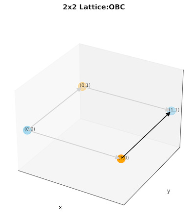
where the black arrow represents the gauge field that remains dynamical after Gauss law is applied, i.e.
$$\eqalign{- E_{00x} - E_{00y} - q_{00} &= 0 \ E_{00y} - E_{01x} - q_{01} &= 0 \ E_{00x} - E_{10y} - q_{10} &= 0 \ E_{01x} + E_{10y} - q_{11} &= 0 \ q_{00} + q_{01} + q_{10} + q_{11} &= 0. }$$
After this step, the Hamiltonian will be:
$$ H_{E} = \frac{g^{2} \left(E_{10y}^{2} + \left(- E_{10y} + q_{11}\right)^{2} + \left(E_{10y} + q_{10}\right)^{2} + \left(- E_{10y} + q_{01} + q_{11}\right)^{2}\right)}{2} $$
for the electric part,
$$ H_{B} = - \frac{U_{10y} + h.c.}{2 g^{2}} $$
for magnetic. If matter fields are considered, then we have a mass term
$$ H_{m} = m \left(\Phi_{1}^{\dagger} \Phi_{1} - \Phi_{2}^{\dagger} \Phi_{2} + \Phi_{3}^{\dagger} \Phi_{3} - \Phi_{4}^{\dagger} \Phi_{4}\right) $$
and a kinetic term
$$ H_{K} = \Omega \left(0.5 i \left(- h.c.(x) + \Phi_{1}^{\dagger} \Phi_{2} + \Phi_{4}^{\dagger} \Phi_{3}\right) - 0.5 \left(h.c.(y) + \Phi_{1}^{\dagger} \Phi_{4} - \Phi_{2}^{\dagger} U_{10y}^{\dagger} \Phi_{3}\right)\right). $$
One can visualize the Hamiltonian and then decide which encoding to use and if the final expression must be written in terms of Qiskit's Pauli operators.
It is also possible to put static charges on the sites and study the static potential.
To encode the fermions for a quantum circuit implementation we consider the Jordan-Wigner formulation with:
$$ \begin{aligned}\Phi_j &= \prod_{k} (-i\sigma^z_k) \sigma^{+}_j , \quad \text{where } k < j, \end{aligned} $$
$$ \begin{aligned}\Phi_j^{\dagger}&= \prod_{k} (i\sigma^z_k) \sigma^{-}_j, \quad \text{where } k < j. \end{aligned} $$
The dynamical charges can be written as
$$q_{\vec{n}} = \Phi^{\dagger} \Phi-\frac{1}{2}(1+(-1)^{n_{x} +n_{y} + 1}) \ \to \ \ \begin{cases} \frac{I-\sigma_{z}}{2}, & \text{if $\vec{n}$ even}\ -\frac{I+\sigma_{z}}{2}, & \text{if $\vec{n}$ odd} \end{cases}$$
Gray circuit
After discretizing and truncating the U(1) gauge group to the discrete group Z(2l+1), the gauge fields can be represented in the electric basis as
$$ \hat{E} = \sum_{i=-l}^l i \ket{i}\bra{i}, $$
$$ \hat{U} = \sum_{i=-l}^{l-1} \ket{i+1}\bra{i}, $$
$$ \hat{U^\dagger} = \sum_{i=-l+1}^l \ket{i-1}\bra{i}, $$
$$\text{where}\ket{i}=\ket{i}_{\text{ph}} $$.
For numerical calculations, it is advantageous to employ a suitable encoding that accurately represents the physical values of the gauge fields.
In this work, we consider the Gray encoding.
For the truncation l=1, we can use the circuit in the following Figure to represent a gauge field.
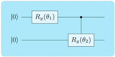
The action of the circuit is straightforward: starting from the state |00>, setting both parameters θ1 and θ2 to zero allows for the exploration of the physical state |-1>. The introduction of a non-zero value for θ1 allows the state to change to |01>, which represents the physical vacuum state |0>, with a certain probability. A complete rotation occurs if θ1 = π, resulting in the exclusive presence of the second state with a probability of 1.0. Subsequently, the second controlled gate operates only when the first qubit is |1>, limiting the exploration to |11> (i.e., physical |1>) and excluding |10>.
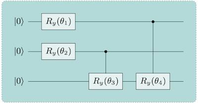
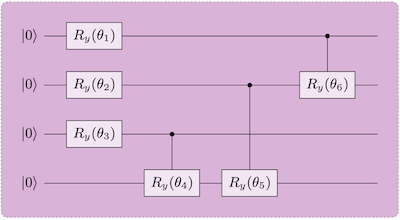
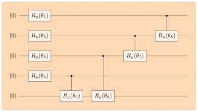
Circuits for larger truncations (l=3,7,15) are:
Fermionic circuit
For simulating the fermionic degrees of freedom we employ the iSWAP gate, see Ref.[^4].
Feedback and Bugs
If any bugs related to installation, usage and workflow are encountered, and in case of suggestions for improvements and new features, please open a New Issue
Contributing
To assist with potential contributions, please submit a Pull Request.
License
References
[^1]: Lattice fermions L Susskind - Physical Review D, 1977 - APS [^2]: P. Jordan and E. P. Wigner, Über das paulische äquivalenzverbot, in The Collected Works of Eugene Paul Wigner (Springer, New York, 1993), pp. 109–129 [^3]: JF Haase, L Dellantonio, A Celi, D Paulson, A Kan, K Jansen, CA Muschik Quantum, 2021•quantum-journal.org [^4]: D. Paulson, L. Dellantonio, J. F. Haase, A. Celi, A. Kan, A. Jena, C. Kokail, R. van Bijnen, K. Jansen, P. Zoller, C. A. Muschik, arXiv:2008.09252
Release history Release notifications | RSS feed


Download files
Download the file for your platform. If you're not sure which to choose, learn more about installing packages.
Source Distribution
Built Distribution
Filter files by name, interpreter, ABI, and platform.
If you're not sure about the file name format, learn more about wheel file names.
Copy a direct link to the current filters
File details
Details for the file qclatticeh-0.1.0rc5.tar.gz.
File metadata
- Download URL: qclatticeh-0.1.0rc5.tar.gz
- Upload date:
- Size: 43.9 kB
- Tags: Source
- Uploaded using Trusted Publishing? No
- Uploaded via: python-httpx/0.28.1
File hashes
| Algorithm | Hash digest | |
|---|---|---|
| SHA256 |
90fe181dde7d323048405d12b66d9b4614c9acd4f9e5b8ece431f04c5be7c5dd
|
|
| MD5 |
d9ec332a9ec4d5b46bb8fec1760f8739
|
|
| BLAKE2b-256 |
48f1a2a59d73e6dbe3c8c7f28779dee47f51bbc3d4a47156f1ebcfd867e8e3cf
|
File details
Details for the file qclatticeh-0.1.0rc5-py3-none-any.whl.
File metadata
- Download URL: qclatticeh-0.1.0rc5-py3-none-any.whl
- Upload date:
- Size: 46.9 kB
- Tags: Python 3
- Uploaded using Trusted Publishing? No
- Uploaded via: python-httpx/0.28.1
File hashes
| Algorithm | Hash digest | |
|---|---|---|
| SHA256 |
da96608ae1843d561169fa2e0ea9cd4b36ad8b8f4f944c2a536cba0eae513fb8
|
|
| MD5 |
c9ab4910660ebb8f81e747d24598da62
|
|
| BLAKE2b-256 |
510a63d3e0fad243a6f627baf4e1468e57ae045278d382f2b56850a0e6c1d632
|


