
qiskit-qaoa-knapsack-domi
Solving the 0/1 knapsack problem by digitized quantum annealing on IBM Quantum hardware. There is no classical optimizer — the cost function parameters are found in advance by statevector-simulating the very circuit that will then run.
Only values, weights and capacity are passed into the module. N is
derived from their count, and the rest of the parameters (ALPHA, LAM1, LAM2,
STEPS, T, recommended SHOTS) are determined by tune_penalties().
Read docs/theory.md before tuning anything by hand. The parameters are not independent.
LAM1andLAM2reshape the energy landscape and, through the normalization, also change how much of the evolution a givenTperforms — so they cannot be set separately fromSTEPSandT. And whichprune_keepvalues are safe depends onLAM1andLAM2in turn: measured sweeps show one instance collapsing across a wide band around 0.7 that another passes straight through. The theory notes derive these relations and give the measured tables.
Documentation
- docs/theory.md — how the knapsack becomes a QUBO, then an
Ising Hamiltonian, then a digitized annealing circuit; coupler pruning and its
cost; and what the Lagrange multipliers
LAM1andLAM2actually do (shadow price, effective capacity, the three failure modes); plus a purely mathematical account of whattune_penalties()computes in preprocessing. - docs/example_output.md — a complete run on
ibm_kingston: job monitoring, time breakdown and the result summary.
The theory notes contain a lot of LaTeX, which GitHub renders but PyPI does not
— that is why they live in docs/ rather than in this file.
Installation
pip install qiskit-qaoa-knapsack-domi          # core
pip install "qiskit-qaoa-knapsack-domi[plots]" # + matplotlib for the plots
pip install "qiskit-qaoa-knapsack-domi[all]"   # + mapomatic
To run on real hardware you need to save your account once:
from qiskit_ibm_runtime import QiskitRuntimeService

QiskitRuntimeService.save_account(
    channel="ibm_quantum_platform",
    token="...",       # from quantum.ibm.com
    instance="crn:v1:bluemix:public:quantum-computing:...",
    overwrite=True, set_as_default=True,
)
Quick start
from qiskit_qaoa_knapsack_domi import KnapsackProblem, RunConfig, solve

problem = KnapsackProblem.random(15, seed=38)      # or your own values/weights
session = solve(problem, config=RunConfig(dry_run=True))

print(session.result.value, "/", session.result.optimum)
Defining the instance
The inputs are always just values, weights and capacity. N is derived
from len(values) and is never given separately.
Your own numbers
problem = KnapsackProblem(
    values=[10, 20, 30, 40],
    weights=[5, 4, 6, 3],
    capacity=10,          # when omitted, sum(weights) // 3 is used
)
Exactly as in the notebook
This notebook code:
import random

random.seed(38)
N = 15
values   = [random.randint(5, 60) for _ in range(N)]
weights  = [random.randint(1, 20) for _ in range(N)]
CAPACITY = sum(weights) // 3
can be carried over in two ways. Either literally, if you want to keep the generation under your own control:
import random
from qiskit_qaoa_knapsack_domi import KnapsackProblem

random.seed(38)
N = 15
values   = [random.randint(5, 60) for _ in range(N)]
weights  = [random.randint(1, 20) for _ in range(N)]
CAPACITY = sum(weights) // 3

problem = KnapsackProblem(values, weights, CAPACITY)
problem.log()
# values : [45, 31, 32, 53, 51, 11, 9, 28, 49, 34, 28, 7, 43, 47, 15]
# weights: [19, 12, 11, 9, 11, 20, 10, 16, 19, 13, 8, 20, 3, 17, 16]
# capacity: 68
Or in short via random(), which gives a bit-for-bit identical instance —
it generates the same sequence with the same generator:
problem = KnapsackProblem.random(15, seed=38)
Setting the capacity by hand
The capacity does not have to be a third of the total weight. It can be given directly:
problem = KnapsackProblem.random(15, seed=38, capacity=100)        # exact value
problem = KnapsackProblem.random(15, seed=38, capacity_divisor=4)  # a quarter
The same applies to KnapsackProblem(...) — capacity is the third positional
argument, and capacity_divisor is used only when you omit it:
KnapsackProblem(values, weights, 100)                      # capacity 100
KnapsackProblem(values, weights)                           # sum(weights) // 3
KnapsackProblem(values, weights, capacity_divisor=4)       # sum(weights) // 4
The capacity must be positive and smaller than the total weight; otherwise everything would fit and the instance would be trivial.
Different random ranges
problem = KnapsackProblem.random(
    20, seed=7,
    value_range=(5, 60),      # both bounds inclusive
    weight_range=(1, 20),
    capacity=120,
)
From the command line:
qiskit-qaoa-knapsack-domi --n 15 --seed 38 --capacity 100
qiskit-qaoa-knapsack-domi --values 10,20,30 --weights 5,4,6 --capacity 9
Settings (RunConfig)
The equivalent of the notebook's SETTINGS block. Original names in comments:
from qiskit_qaoa_knapsack_domi import RunConfig, PlotConfig

cfg = RunConfig(
    dry_run=False,          # DRY_RUN: True = local fake backend (free)
    opt_level=3,            # OPT_LEVEL: transpiler aggressiveness
    num_transpiles=10,      # NUM_TRANSPILES: how many seeds to score
    use_mapomatic=False,    # USE_MAPOMATIC
    make_plots=True,        # MAKE_PLOTS: layout + result plots
    draw_circuit=True,      # DRAW_CIRCUIT: circuit diagrams
    fold=100,               # FOLD: gates per row (-1 = one row)
    layout_view="physical", # LAYOUT_VIEW: "physical" | "virtual"
    prune_keep=0.5,         # PRUNE_KEEP: fraction of ZZ couplings kept
    shots=300_000,          # SHOTS; "auto" = take tune_penalties' recommendation
    plots=PlotConfig(save_dir="out"),   # where to save the PNGs
)
There is no N in RunConfig — it comes from len(problem.values).
Step by step
solve() is only a wrapper; every step can be called on its own:
from qiskit_qaoa_knapsack_domi import (
    KnapsackProblem, RunConfig, PlotConfig, tune_penalties,
    build_annealing_circuit, select_backend, transpile_best, run_circuit,
    build_result, build_distribution, plot_bitstrings, plot_tail,
)

problem = KnapsackProblem.random(15, seed=38)
cfg = RunConfig(
    dry_run=True,
    prune_keep=0.5,
    draw_circuit=True,               # logical and ISA circuit diagrams
    make_plots=True,                 # coupling map
    plots=PlotConfig(save_dir="out"),
)

# 1) penalties: ALPHA, LAM1, LAM2, STEPS, T + recommended SHOTS
pen = tune_penalties(
    problem,
    schedule_grid=[(3, 6.0), (5, 10.0), (7, 15.0)],
    max_rzz=500,
    alpha_out=2.0,
    l1_range=(2.0, 25.0),     # None = automatic window around the LP dual
    l2_range=(0.1, 5.0),
)
ALPHA, LAM1, LAM2, STEPS, T = pen.as_tuple()

# 2) QUBO -> ZZ pruning -> Ising -> circuit
#    draws the circuit diagram itself when draw_circuit=True
qc, qubo, ising = build_annealing_circuit(problem, penalties=pen, config=cfg)

# 3) backend + noise-aware transpilation
#    draws the coupling map and ISA diagram per make_plots / draw_circuit
backend = select_backend(cfg, num_qubits=qubo.n)
tr = transpile_best(qc, backend, cfg, num_items=problem.n)

# 4) run
counts = run_circuit(tr.circuit, backend, cfg, pen)

# 5) results -- build_result prints the RESULT SUMMARY block
result = build_result(counts, problem, backend=backend, transpiled=tr)
dist = build_distribution(counts, problem, good=0.90)

# 6) result plots are called by hand; `plots=` is needed to save the PNGs
plot_bitstrings(dist, backend_name=backend.name, plots=cfg.plots)
plot_tail(dist, plots=cfg.plots)
What gets drawn when
draw_circuit and make_plots behave the same in solve() and step by step:
| flag | what it draws | where |
|---|---|---|
draw_circuit |
logical circuit diagram | build_annealing_circuit() |
draw_circuit |
ISA circuit diagram (what runs on the chip) | transpile_best() |
make_plots |
coupling map with the used qubits highlighted | transpile_best() |
The result plots (plot_bitstrings, plot_tail) are drawn by solve() itself
when make_plots=True. Going step by step you call them yourself — and if you
also want them saved, pass plots=cfg.plots, otherwise they are only displayed.
Printing the result summary
The KNAPSACK - RESULT SUMMARY table is printed by solve() after the run.
Step by step, build_result does it:
result = build_result(counts, problem, backend=backend, transpiled=tr)
print(result.value, result.optimum, result.is_optimal)
Pass backend= and transpiled= so the header can show the backend name, the
layout method and the two-qubit gate count; without them those fields are
blank. verbose=False returns the KnapsackResult without printing anything.
The job monitor (Job ID, the state timeline and TIME BREAKDOWN) comes from
run_circuit and only runs on real hardware — in dry_run there is no job to
follow.
What tune_penalties does
It searches (LAM1, LAM2) pairs and (STEPS, T) schedules and picks the ones with the highest P(optimum). Scoring is always a statevector simulation of the circuit that will then run — no proxy quantity.
- Hard condition: pairs where the global minimum of the cost function is not the DP optimum are discarded. This is tested on a Pareto reduction, i.e. on a few hundred candidates instead of 2^N.
- Coarse grid → refinement → final: phases A/B run the cheapest schedule,
and all schedules are tried only on the
n_finalbest candidates. - LAM2 is traversed logarithmically — the optimum often sits just above the validity floor, where a linear grid has no resolution.
l1_range=Noneturns on an automatic window around the LP dual (the shadow price of capacity). Measured on N=8..15: the winning LAM1/ALPHA always fell within 1.09–1.38× the LP dual.gate_error=...scores P(opt) after the attenuationexp(-gate_error * 2.9 * RZZ), so a depth the hardware cannot sustain is not selected.
It returns Penalties, which can also be indexed like a dictionary
(pen["LAM1"]), so code carried over from the notebook works unchanged.
The original slow tune_penalties from the notebook is not part of the package;
only the fast version (tune_penalties2 in the notebook) remains, under the
name without the digit.
Pruning the couplings
prune_keep is the main lever on circuit depth — weak couplings cost just as
many two-qubit gates as strong ones. It can also be called on its own:
from qiskit_qaoa_knapsack_domi import prune_couplings

quad = prune_couplings(raw_couplings, prune_keep=0.5)
# ZZ gates: stayed 53/105 (50%)
Pruning is not only a compromise. On the reference instance prune_keep=0.5
samples the optimum four times more strongly than the complete model, while
using half the RZZ and therefore decohering less on hardware.
Use 1.0 or 0.5; below that, verify. Measured on three instances, 0.5 is at
least as good as 1.0 everywhere and uses half the RZZ. Lower values are not
safe to extrapolate to: quality degrades below roughly 0.3–0.4 on every instance
tested, and one instance collapses across a wide band around 0.7 that another
sails straight through. Which values misbehave depends on LAM1 and LAM2, so
the three have to be judged together. The sweeps are in
docs/theory.md.
Plots
Plotting is kept separate so the package can be used without matplotlib:
| function | what it does |
|---|---|
draw_circuit_diagram(qc, cfg) |
diagram of the logical or transpiled circuit |
plot_layout(isa, backend, cfg) |
coupling map with the used qubits highlighted |
plot_bitstrings(dist) |
top-K bitstrings; red = optimum, blue = within 10 % |
plot_tail(dist) |
P(sample at least this good) vs uniform random |
plot_results(counts, problem) |
both at once from ready-made counts |
How many bitstrings to plot
plot_bitstrings draws the K most probable bitstrings, 300 by default. Two
ways to change that — a per-call argument, or the config:
# per call; overrides the config without modifying it
plot_bitstrings(dist, backend_name=backend.name, top_k=50, plots=cfg.plots)

# or as a default for the whole run, including inside solve()
cfg = RunConfig(plots=PlotConfig(top_k=50, save_dir="out"))
plot_results takes top_k as well. Bitstrings that were never sampled are
dropped, so with top_k=300 and only 80 distinct outcomes you get 80 bars.
The figure width scales with the number of bars (clamped between 14 and 50
inches), so large values produce very wide images — for a readable chart 30–100
usually works better than the default.
Command line
qiskit-qaoa-knapsack-domi --n 15 --seed 38 --dry-run --no-draw
qiskit-qaoa-knapsack-domi --values 10,20,30 --weights 5,4,6 --capacity 9 \
    --shots auto --save-dir out --json result.json
Notes on the limits
tune_penaltiesand the ground-state check walk all 2^N states. Above ~20 qubits this stops paying off; the check is skipped automatically abovemax_exact_n(24 by default).- The number of RZZ per layer is N(N−1)/2. At N=15 with STEPS=3 that is 315
logical RZZ before transpilation even starts — hence
max_rzzandprune_keep. - Above
max_twoq_warn(3000) two-qubit gates a warning is printed; by then the result tends to be mostly noise.
Publishing to PyPI
pip install build twine
python -m build          # creates dist/*.whl and dist/*.tar.gz
python -m twine check dist/*
python -m twine upload --repository testpypi dist/*   # TestPyPI first
python -m twine upload dist/*
Before uploading, set the real repository URL and author name in
pyproject.toml.
Development
pip install -e ".[dev]"
pytest -q
ruff check src tests examples
License
Noncommercial use only. Research, experiment, teaching, personal study and hobby projects are permitted purposes, as is use by charitable organizations, educational institutions, public research organizations and government institutions — regardless of how they are funded. Commercial use is not covered; contact the licensor for a separate license.
This is a source-available licence, not an open-source one — it is not OSI
approved, so the package carries no License :: OSI Approved classifier.
The licence grants a patent license for claims the licensor can license and that you would infringe by using the software, and it terminates that patent license if you assert a patent claim against the software.
If you redistribute any part of this package, you must pass on both the licence
terms (or the URL above) and the Required Notice: line. Both ship inside the
wheel at qiskit_qaoa_knapsack_domi-<version>.dist-info/licenses/LICENSE.
Results on real hardware
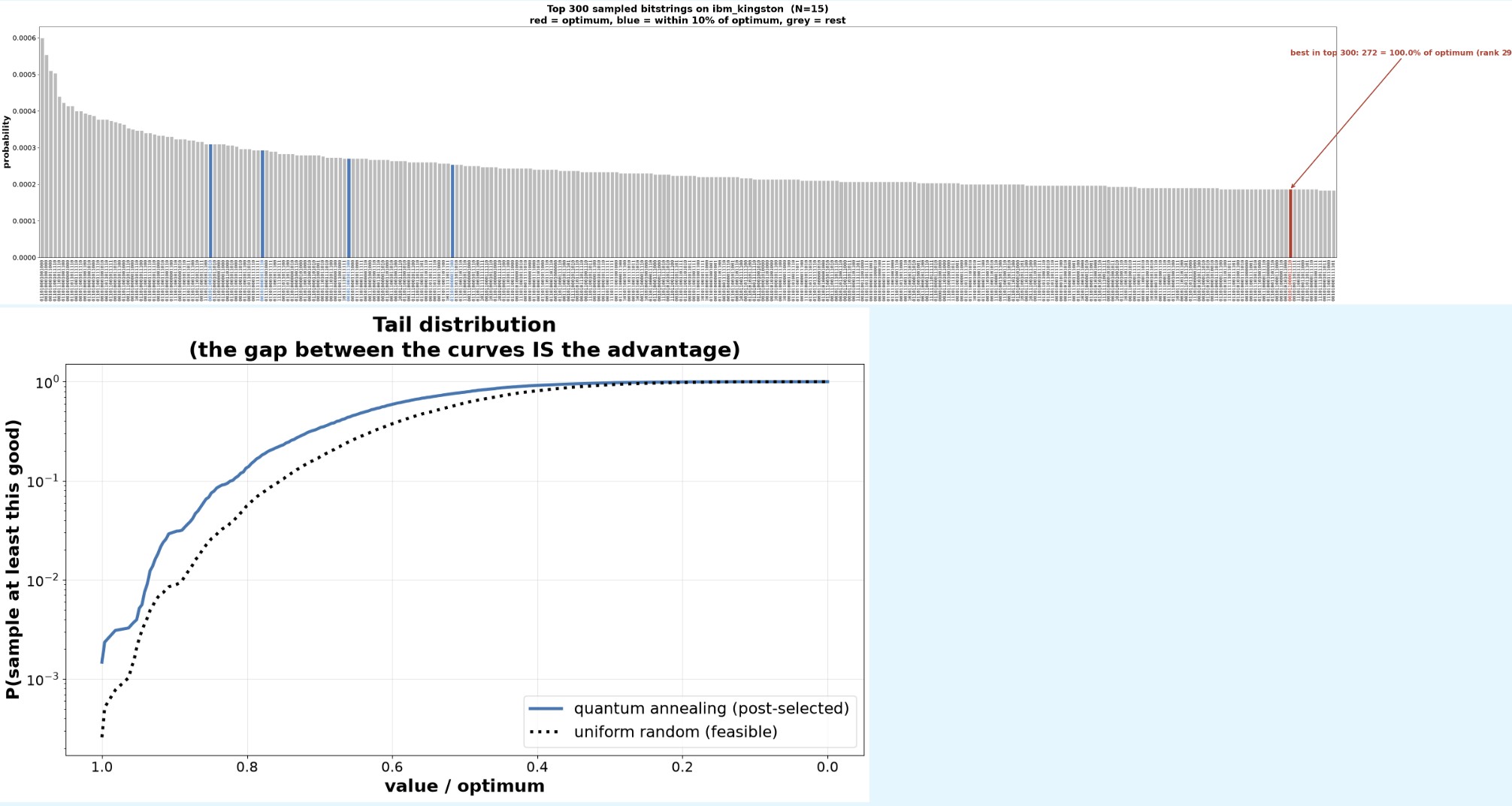
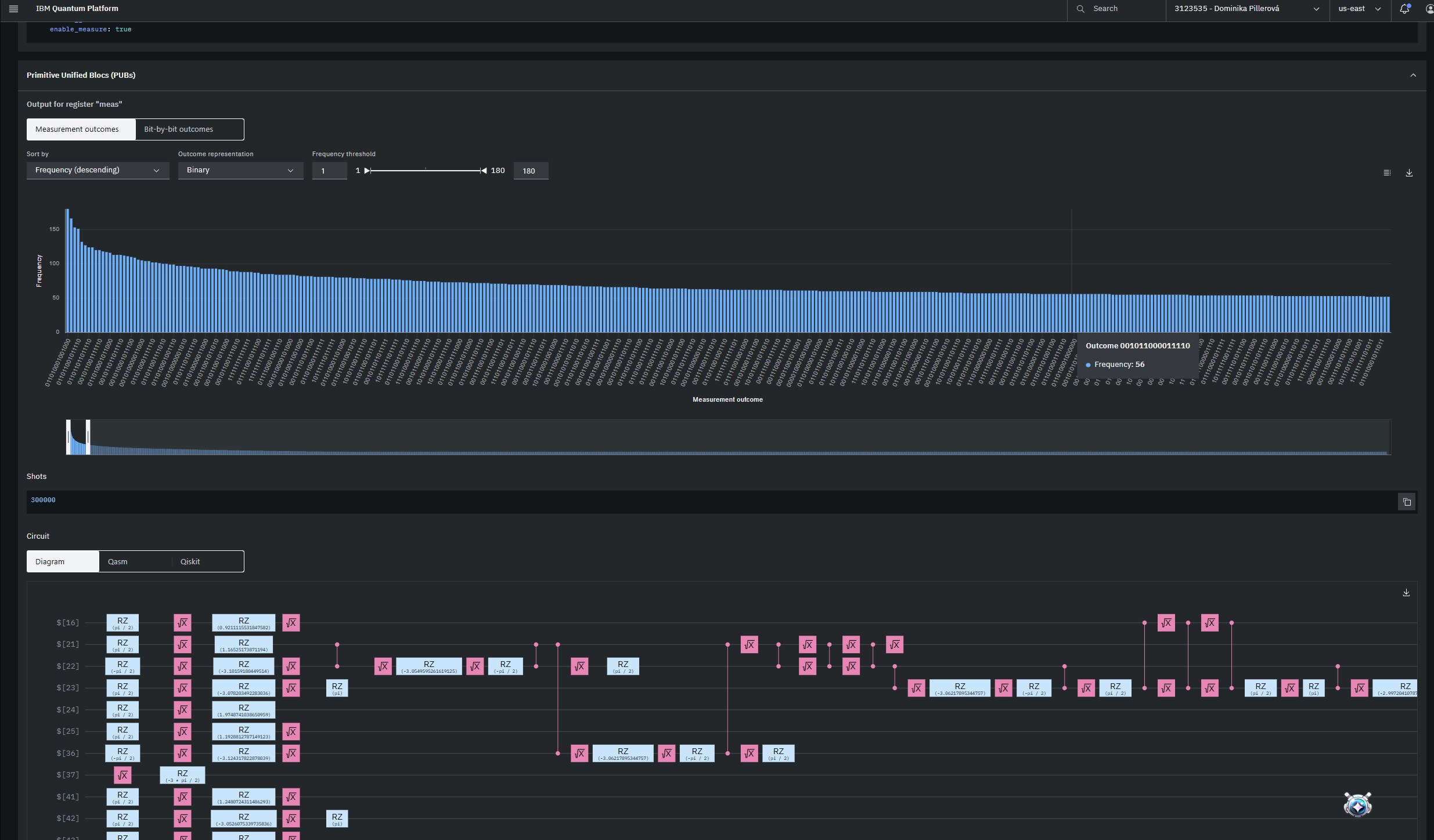
Both plots come from an actual ibm_kingston run of the reference instance —
not a simulator. Red is the optimum, blue is everything within 10 % of it, and
the gap between the two curves in the second plot is the whole point of the
exercise.
Run it yourself and your own optimum will be waiting in outputs/, sampled off
real superconducting qubits. It even beat the DP solver to the answer — well,
"beat" in the sense of arriving at the same 272 rather more expensively.
1 maintainer

Download files
Download the file for your platform. If you're not sure which to choose, learn more about installing packages.
Source Distribution
Built Distribution
Filter files by name, interpreter, ABI, and platform.
If you're not sure about the file name format, learn more about wheel file names.
Copy a direct link to the current filters
File details
Details for the file qiskit_qaoa_knapsack_domi-0.4.2.tar.gz.
File metadata
- Download URL: qiskit_qaoa_knapsack_domi-0.4.2.tar.gz
- Upload date:
- Size: 51.8 kB
- Tags: Source
- Uploaded using Trusted Publishing? Yes
- Uploaded via:
twine/7.0.0 CPython/3.13.14
File hashes
| Algorithm | Hash digest | |
|---|---|---|
| SHA256 |
36e1eef790c169113ee5cd71e0739e82ee06f374507bab131f39ec1615482aac
|
|
| MD5 |
767573352898bd0df06eaa4c5dbda6cd
|
|
| BLAKE2b-256 |
a2baf1cb003a1b114d162a5de0cab815ff7efaa4e143b326ab8244077e25cf4f
|
Provenance
The following attestation bundles were made for qiskit_qaoa_knapsack_domi-0.4.2.tar.gz:
Publisher:
publish.yml on bluemoondom/qiskit-qaoa-knapsack-domi
-
Statement:
-
Statement type:
https://in-toto.io/Statement/v1 -
Predicate type:
https://docs.pypi.org/attestations/publish/v1 -
Subject name:
qiskit_qaoa_knapsack_domi-0.4.2.tar.gz -
Subject digest:
36e1eef790c169113ee5cd71e0739e82ee06f374507bab131f39ec1615482aac - Sigstore transparency entry: 2739108560
- Sigstore integration time:
-
Permalink:
bluemoondom/qiskit-qaoa-knapsack-domi@b5da740834713e00fe312e8f12ad5f49e1374a52 -
Branch / Tag:
refs/heads/main - Owner: https://github.com/bluemoondom
-
Access:
public
-
Token Issuer:
https://token.actions.githubusercontent.com -
Runner Environment:
github-hosted -
Publication workflow:
publish.yml@b5da740834713e00fe312e8f12ad5f49e1374a52 -
Trigger Event:
workflow_dispatch
-
Statement type:
File details
Details for the file qiskit_qaoa_knapsack_domi-0.4.2-py3-none-any.whl.
File metadata
- Download URL: qiskit_qaoa_knapsack_domi-0.4.2-py3-none-any.whl
- Upload date:
- Size: 41.2 kB
- Tags: Python 3
- Uploaded using Trusted Publishing? Yes
- Uploaded via:
twine/7.0.0 CPython/3.13.14
File hashes
| Algorithm | Hash digest | |
|---|---|---|
| SHA256 |
fb527231b5952b62ad4c70996215f662186ccca9eeeab40f534553eb2349ade7
|
|
| MD5 |
b26e0086be4b3596560b607839812bdb
|
|
| BLAKE2b-256 |
acc1b8449c3ebbeb3bff90da6d9c0598cddb9dce2b96f56dfdf9f81c78e0cc53
|
Provenance
The following attestation bundles were made for qiskit_qaoa_knapsack_domi-0.4.2-py3-none-any.whl:
Publisher:
publish.yml on bluemoondom/qiskit-qaoa-knapsack-domi
-
Statement:
-
Statement type:
https://in-toto.io/Statement/v1 -
Predicate type:
https://docs.pypi.org/attestations/publish/v1 -
Subject name:
qiskit_qaoa_knapsack_domi-0.4.2-py3-none-any.whl -
Subject digest:
fb527231b5952b62ad4c70996215f662186ccca9eeeab40f534553eb2349ade7 - Sigstore transparency entry: 2739108647
- Sigstore integration time:
-
Permalink:
bluemoondom/qiskit-qaoa-knapsack-domi@b5da740834713e00fe312e8f12ad5f49e1374a52 -
Branch / Tag:
refs/heads/main - Owner: https://github.com/bluemoondom
-
Access:
public
-
Token Issuer:
https://token.actions.githubusercontent.com -
Runner Environment:
github-hosted -
Publication workflow:
publish.yml@b5da740834713e00fe312e8f12ad5f49e1374a52 -
Trigger Event:
workflow_dispatch
-
Statement type:














