
QOrbit: High-performance numerical/quantum simulation toolkit

Project description






⚛️ QOrbit
A sandbox quantum mechanical simulator
Overview
QOrbit is a Python-based sandbox environment for simulating and visualizing quantum mechanical wavefunctions under arbitrary potential landscapes. In quantum mechanics, physical intuition from classical systems often breaks down. The dynamics of a system are governed by the Schrödinger equation, which becomes increasingly difficult to solve analytically as system complexity grows. Even numerical approaches face severe scalability challenges due to the exponential growth of degrees of freedom and basis size in multi-particle systems. QOrbit addresses this by providing a highly parallelizable numerical framework that uses orthogonal Fourier basis expansions, linear algebra acceleration (BLAS / GEMM routines), and optional GPU acceleration to approximate and analyze quantum states in 2D systems.
Installation
QOrbit can be installed directly from PyPI or from source.
Option 1: Install from PyPI (Recommended)
CPU Version
pip install qorbit
GPU Version
Installs optional GPU acceleration dependencies.
pip install "qorbit[gpu]"
Option 2: Install from Source
Clone the repository and install in editable mode.
git clone https://github.com/abhaskumarsinha/QOrbit.git
cd QOrbit
pip install -e .
For development workflows, editable installation automatically reflects source code changes without requiring reinstallation.
Google Colab Installation
CPU
!pip install qorbit
GPU
!pip install "qorbit[gpu]"
Development Setup
git clone https://github.com/abhaskumarsinha/QOrbit.git
cd QOrbit
pip install -e .
cd src
This setup is recommended for:
- Contributing to QOrbit
- Developing custom solvers
- Modifying basis functions
- Experimenting with new potential models
Requirements
- Python 3.10+
- NumPy
- SciPy
- Matplotlib
Optional:
- CuPy (GPU acceleration)
- NVIDIA CUDA-compatible/AMD Ryzen/Intel Graphics Driver GPU
Verify Installation
import qorbit

print("QOrbit installed successfully!")
Key Idea
Instead of attempting exact solutions, QOrbit constructs an approximate representation of the wavefunction using:
- Fourier basis decomposition
- Slater determinant construction (fermionic states)
- Numerical diagonalization of the Hamiltonian
- Efficient matrix operations for large-scale basis evaluation
This allows scalable approximation of stationary states in complex potential landscapes.
Features
-
🧠 Custom potential landscapes
- Define arbitrary potential energy functions: wells, barriers, charges, particles, obstacles, or maze-like geometries.
-
⚡ Fast numerical solver
- Uses optimized BLAS (GEMM) operations for matrix construction and diagonalization.
-
🧮 Fourier basis expansion
- Represents wavefunctions in orthogonal Fourier space for efficient convergence.
-
🧱 Slater determinant framework
- Supports fermionic multi-particle state construction (currently spinless).
-
📊 Wavefunction visualization
- Compute and visualize:
- Probability densities
- Marginal distributions
- Conditional distributions (where applicable)
- Compute and visualize:
-
🚀 Parallelizable design
- Core routines are structured for GPU acceleration and batch evaluation.
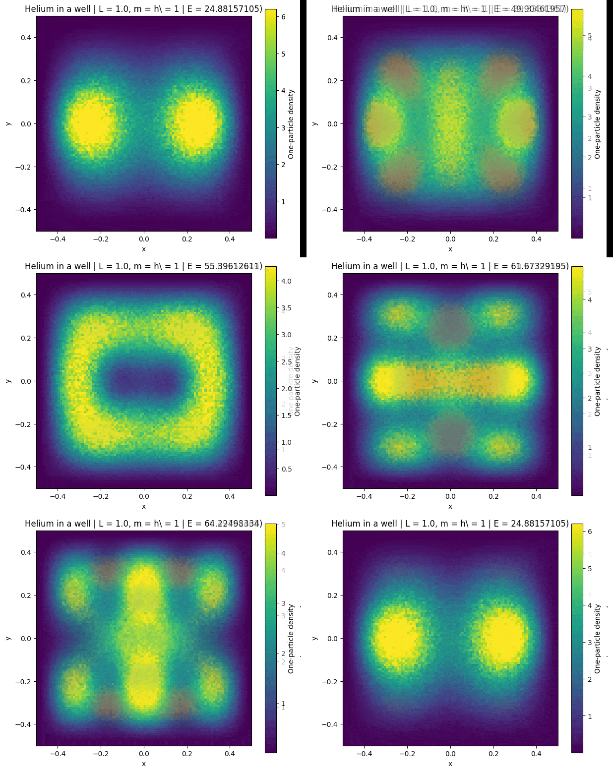
Current Limitations
- Only supports non-relativistic, spinless fermionic systems
- Restricted to 2D square-well-like domains
- No built-in many-body correlation beyond Slater determinant structure (mean-field-like approximation)
- GPU support depends on available backend configuration
Future extensions may include:
- Spinful fermions
- Bosonic systems
- Time-dependent Schrödinger evolution
- Improved correlation methods beyond determinant basis
Simulation Performance
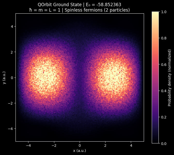
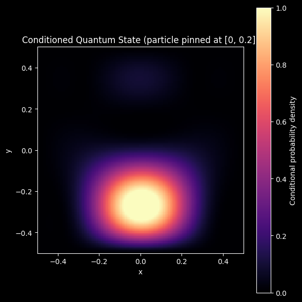
- In CPU
Intel(R) Xeon(R) CPU @ 2.20GHzsingle thread over numpy.
🔬 Full simulation code (click to expand)
import time
import numpy as np
import matplotlib.pyplot as plt

from qorbit import (
    generate_slater_determinants,
    build_hamiltonian,
    diagonalize_hamiltonian,
    build_ci_states,
    density_grid,
    conditional_density_grid
)

from qorbit.potentials import create_potential


# ============================================================
# SCI-FI VISUAL CONFIG
# ============================================================
plt.style.use("dark_background")
CMAP = "magma"


def timer(label, t0):
    dt = time.time() - t0
    print(f"[⏱] {label:<40} {dt:8.4f} s")
    return dt


TOTAL_T0 = time.time()


# ============================================================
# 1. SLATER DETERMINANTS
# ============================================================
t0 = time.time()

Phi_list, det_energies, det_pairs = generate_slater_determinants(
    num_particles=2,
    max_orbital=10,
    xp=np
)

timer("Slater determinant generation", t0)


# ============================================================
# 2. POTENTIAL (FIXED: h2 instead of H2Potential)
# ============================================================
t0 = time.time()

V_func = create_potential(
    "h2",
    Z=5.0,
    k_coulomb=1.0,
    xp=np
)

timer("Potential construction (H2 model)", t0)


# ============================================================
# 3. HAMILTONIAN BUILD
# ============================================================
t0 = time.time()

H = build_hamiltonian(
    Phi_list=Phi_list,
    det_energies=det_energies,
    potential_fn=V_func,
    n_particles=2,
    L=1.0,
    num_samples=800_000,
    seed=123,
    k_coulomb=1.0,
    xp=np
)

timer("Hamiltonian assembly", t0)


# ============================================================
# 4. DIAGONALIZATION
# ============================================================
t0 = time.time()

energies, eigenvectors = diagonalize_hamiltonian(H, xp=np)

timer("Hamiltonian diagonalization", t0)


# ============================================================
# 5. CI STATES
# ============================================================
t0 = time.time()

CI_states = build_ci_states(Phi_list, eigenvectors, xp=np)

ground_state = CI_states[0]
ground_energy = energies[0]

timer("CI state reconstruction", t0)


# ============================================================
# 6. DENSITY (MONTE CARLO)
# ============================================================
print("\n[🌌] Computing quantum probability density...")

t0 = time.time()

X, Y, rho = density_grid(
    psi=ground_state,
    n_particles=2,
    L=1.0,
    grid_size=140,
    mc_samples=120,
    seed=42,
    xp=np
)

timer("MC density evaluation", t0)


# ============================================================
# NORMALIZATION (IMPORTANT FOR VISUAL QUALITY)
# ============================================================
rho = np.array(rho)

vmin, vmax = np.percentile(rho, [2, 98])
rho = np.clip((rho - vmin) / (vmax - vmin + 1e-12), 0, 1)

# gamma boost → reveals orbital structure
rho = rho ** 0.55


# ============================================================
# 7. MAIN DENSITY PLOT
# ============================================================
plt.figure(figsize=(7, 6))

plt.imshow(
    rho,
    origin="lower",
    extent=[-5, 5, -5, 5],
    cmap=CMAP,
    aspect="equal"
)

plt.colorbar(label="Probability density (normalized)")

plt.title(
    f"QOrbit Ground State | E₀ = {ground_energy:.6f}\n"
    "ħ = m = L = 1 | Spinless fermions (2 particles)"
)

plt.xlabel("x (a.u.)")
plt.ylabel("y (a.u.)")

plt.tight_layout()
plt.show()


# ============================================================
# 8. ZOOM VIEW (ORBITAL STRUCTURE)
# ============================================================
plt.figure(figsize=(6, 6))

plt.imshow(
    rho,
    origin="lower",
    extent=[-0.5, 0.5, -0.5, 0.5],
    cmap=CMAP,
    aspect="equal"
)

plt.colorbar(label="Density (zoomed)")

plt.title("Quantum Core Structure (high-resolution orbital shape)")
plt.xlabel("x")
plt.ylabel("y")

plt.tight_layout()
plt.show()


# ============================================================
# 9. CONDITIONAL DENSITY (CORRELATION VIEW)
# ============================================================
t0 = time.time()

X, Y, cond = conditional_density_grid(
    psi=ground_state,
    n_particles=2,
    L=1.0,
    fixed_indices=[0],
    fixed_positions=np.array([[0.1, 0.0]]),
    target_index=1,
    grid_size=120,
    mc_samples=80,
    seed=42,
    chunk_size=512
)

timer("Conditional density", t0)


# ============================================================
# VISUALIZE CONDITIONAL STRUCTURE
# ============================================================
cond = np.array(cond)

vmin, vmax = np.percentile(cond, [2, 98])
cond = np.clip((cond - vmin) / (vmax - vmin + 1e-12), 0, 1)
cond = cond ** 0.6

plt.figure(figsize=(6, 6))

plt.imshow(
    cond,
    origin="lower",
    extent=[-0.5, 0.5, -0.5, 0.5],
    cmap=CMAP,
    aspect="equal"
)

plt.colorbar(label="Conditional probability density")

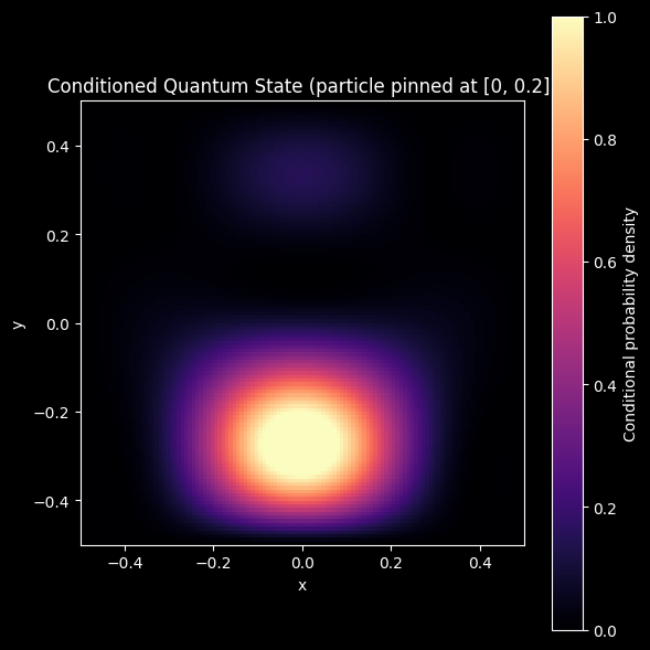
plt.title("Conditioned Quantum State (particle pinned at [0, 0.2])")
plt.xlabel("x")
plt.ylabel("y")

plt.tight_layout()
plt.show()


# ============================================================
# 10. FINAL REPORT
# ============================================================
TOTAL_TIME = time.time() - TOTAL_T0

print("\n" + "=" * 60)
print(" QORBIT SIMULATION REPORT")
print("=" * 60)
print(f"Ground state energy : {ground_energy:.8f}")
print(f"Particles           : 2 (spinless fermions)")
print(f"Basis size          : {len(Phi_list)}")
print(f"Domain              : L = 1.0 (2D box)")
print(f"MC samples          : 800k (Hamiltonian), 120 (density)")
print(f"Total runtime       : {TOTAL_TIME:.3f} s")
print("=" * 60)
[⏱] Slater determinant generation              0.0007 s
[⏱] Potential construction (H2 model)          0.0001 s
Evaluating wavefunctions on batch...
Evaluating potential on batch...
[⏱] Hamiltonian assembly                      25.0820 s
[⏱] Hamiltonian diagonalization                0.0014 s
[⏱] CI state reconstruction                    0.0006 s

[🌌] Computing quantum probability density...
Density grid (chunks): 100%|██████████| 77/77 [01:03<00:00,  1.22chunk/s]
[⏱] MC density evaluation                     63.2278 s
Conditional density: 100%|██████████| 29/29 [00:27<00:00,  1.07chunk/s]
[⏱] Conditional density                       27.2310 s

============================================================
 QORBIT SIMULATION REPORT
============================================================
Ground state energy : -58.85236329
Particles           : 2 (spinless fermions)
Basis size          : 55
Domain              : L = 1.0 (2D box)
MC samples          : 800k (Hamiltonian), 120 (density)
Total runtime       : 116.311 s
============================================================
- In GPU
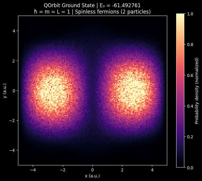
T4 Tesla
🔬 Full simulation code (click to expand)
import time
import cupy as np
import matplotlib.pyplot as plt

from qorbit import (
    generate_slater_determinants,
    build_hamiltonian,
    diagonalize_hamiltonian,
    build_ci_states,
    density_grid,
    conditional_density_grid
)

from qorbit.potentials import create_potential


# ============================================================
# SCI-FI VISUAL CONFIG
# ============================================================
plt.style.use("dark_background")
CMAP = "magma"


def timer(label, t0):
    dt = time.time() - t0
    print(f"[⏱] {label:<40} {dt:8.4f} s")
    return dt


TOTAL_T0 = time.time()


# ============================================================
# 1. SLATER DETERMINANTS
# ============================================================
t0 = time.time()

Phi_list, det_energies, det_pairs = generate_slater_determinants(
    num_particles=2,
    max_orbital=10,
    xp=np
)

timer("Slater determinant generation", t0)


# ============================================================
# 2. POTENTIAL (FIXED: h2 instead of H2Potential)
# ============================================================
t0 = time.time()

V_func = create_potential(
    "h2",
    Z=5.0,
    k_coulomb=1.0,
    xp=np
)

timer("Potential construction (H2 model)", t0)


# ============================================================
# 3. HAMILTONIAN BUILD
# ============================================================
t0 = time.time()

H = build_hamiltonian(
    Phi_list=Phi_list,
    det_energies=det_energies,
    potential_fn=V_func,
    n_particles=2,
    L=1.0,
    num_samples=800_000,
    seed=123,
    k_coulomb=1.0,
    xp=np
)

timer("Hamiltonian assembly", t0)


# ============================================================
# 4. DIAGONALIZATION
# ============================================================
t0 = time.time()

energies, eigenvectors = diagonalize_hamiltonian(H, xp=np)

timer("Hamiltonian diagonalization", t0)


# ============================================================
# 5. CI STATES
# ============================================================
t0 = time.time()

CI_states = build_ci_states(Phi_list, eigenvectors, xp=np)

ground_state = CI_states[0]
ground_energy = energies[0]

timer("CI state reconstruction", t0)


# ============================================================
# 6. DENSITY (MONTE CARLO)
# ============================================================
print("\n[🌌] Computing quantum probability density...")

t0 = time.time()

X, Y, rho = density_grid(
    psi=ground_state,
    n_particles=2,
    L=1.0,
    grid_size=140,
    mc_samples=120,
    seed=42,
    xp=np
)

timer("MC density evaluation", t0)


# ============================================================
# NORMALIZATION (IMPORTANT FOR VISUAL QUALITY)
# ============================================================
rho = np.array(rho)

vmin, vmax = np.percentile(rho, [2, 98])
rho = np.clip((rho - vmin) / (vmax - vmin + 1e-12), 0, 1)

# gamma boost → reveals orbital structure
rho = rho ** 0.55


# ============================================================
# 7. MAIN DENSITY PLOT
# ============================================================
plt.figure(figsize=(7, 6))

rho = np.asnumpy(rho)

plt.imshow(
    rho,
    origin="lower",
    extent=[-5, 5, -5, 5],
    cmap=CMAP,
    aspect="equal"
)

plt.colorbar(label="Probability density (normalized)")

plt.title(
    f"QOrbit Ground State | E₀ = {ground_energy:.6f}\n"
    "ħ = m = L = 1 | Spinless fermions (2 particles)"
)

plt.xlabel("x (a.u.)")
plt.ylabel("y (a.u.)")

plt.tight_layout()
plt.show()


# ============================================================
# 8. ZOOM VIEW (ORBITAL STRUCTURE)
# ============================================================
plt.figure(figsize=(6, 6))

rho = np.asnumpy(rho)

plt.imshow(
    rho,
    origin="lower",
    extent=[-0.5, 0.5, -0.5, 0.5],
    cmap=CMAP,
    aspect="equal"
)

plt.colorbar(label="Density (zoomed)")

plt.title("Quantum Core Structure (high-resolution orbital shape)")
plt.xlabel("x")
plt.ylabel("y")

plt.tight_layout()
plt.show()


# ============================================================
# 9. CONDITIONAL DENSITY (CORRELATION VIEW)
# ============================================================
t0 = time.time()

X, Y, cond = conditional_density_grid(
    psi=ground_state,
    n_particles=2,
    L=1.0,
    fixed_indices=[0],
    fixed_positions=np.array([[0.1, 0.0]]),
    target_index=1,
    grid_size=120,
    mc_samples=80,
    seed=42,
    chunk_size=512
)

timer("Conditional density", t0)


# ============================================================
# VISUALIZE CONDITIONAL STRUCTURE
# ============================================================
cond = np.array(cond)

vmin, vmax = np.percentile(cond, [2, 98])
cond = np.clip((cond - vmin) / (vmax - vmin + 1e-12), 0, 1)
cond = cond ** 0.6

plt.figure(figsize=(6, 6))

cond = np.asnumpy(cond)

plt.imshow(
    cond,
    origin="lower",
    extent=[-0.5, 0.5, -0.5, 0.5],
    cmap=CMAP,
    aspect="equal"
)

plt.colorbar(label="Conditional probability density")

plt.title("Conditioned Quantum State (particle pinned at [0, 0.2])")
plt.xlabel("x")
plt.ylabel("y")

plt.tight_layout()
plt.show()


# ============================================================
# 10. FINAL REPORT
# ============================================================
TOTAL_TIME = time.time() - TOTAL_T0

print("\n" + "=" * 60)
print(" QORBIT SIMULATION REPORT")
print("=" * 60)
print(f"Ground state energy : {ground_energy:.8f}")
print(f"Particles           : 2 (spinless fermions)")
print(f"Basis size          : {len(Phi_list)}")
print(f"Domain              : L = 1.0 (2D box)")
print(f"MC samples          : 800k (Hamiltonian), 120 (density)")
print(f"Total runtime       : {TOTAL_TIME:.3f} s")
print("=" * 60)
[⏱] Slater determinant generation              0.0053 s
[⏱] Potential construction (H2 model)          0.0007 s
Evaluating wavefunctions on batch...
Evaluating potential on batch...
[⏱] Hamiltonian assembly                       0.9458 s
[⏱] Hamiltonian diagonalization                0.4256 s
[⏱] CI state reconstruction                    0.0022 s

[🌌] Computing quantum probability density...
Density grid (chunks): 100%|██████████| 77/77 [00:07<00:00, 10.62chunk/s]
[⏱] MC density evaluation                      7.2522 s
Conditional density: 100%|██████████| 29/29 [00:02<00:00, 10.17chunk/s]
[⏱] Conditional density                        2.8561 s

============================================================
 QORBIT SIMULATION REPORT
============================================================
Ground state energy : -61.49276136
Particles           : 2 (spinless fermions)
Basis size          : 55
Domain              : L = 1.0 (2D box)
MC samples          : 800k (Hamiltonian), 120 (density)
Total runtime       : 12.165 s
============================================================
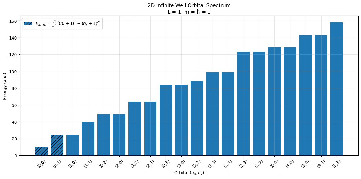
⚛️ Energy & Stability Validation
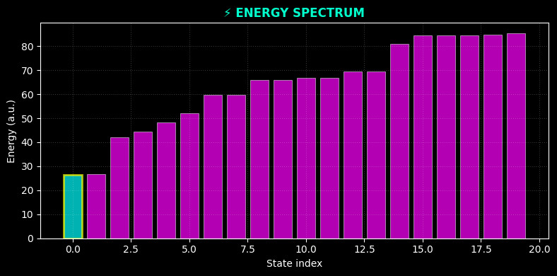
(1) Energy spectrum validation: analytical fermionic 2D box energy levels vs QOrbit CI simulation showing near-exact matching of lower order excited-state structure and correct ordering of quantized levels with deviations only from Monte Carlo sampling noise and finite Fourier basis truncation. The divergence is only at higher energy values that requires more basis expansion.
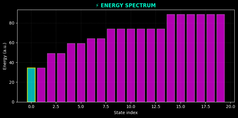
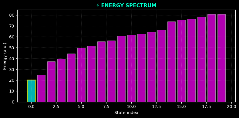
(2) Stability comparison: H₂ potential vs hydron (single proton centered system) inside L=1.0 square well showing that H₂ configuration yields stronger localization and lower total energy indicating higher binding stability compared to hydron case due to stronger Coulomb interaction and electron sharing effect
[Two proton - Two electron system (left)] [Two protons separated at a distance (right)]
Qualitative Results
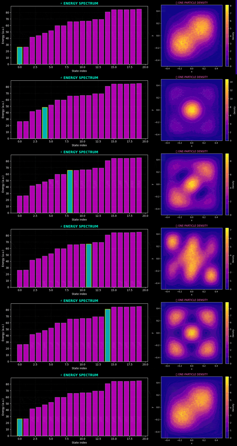 [Two electrons in a well of side L = 1.0 with two fixed protons separated by a distance]
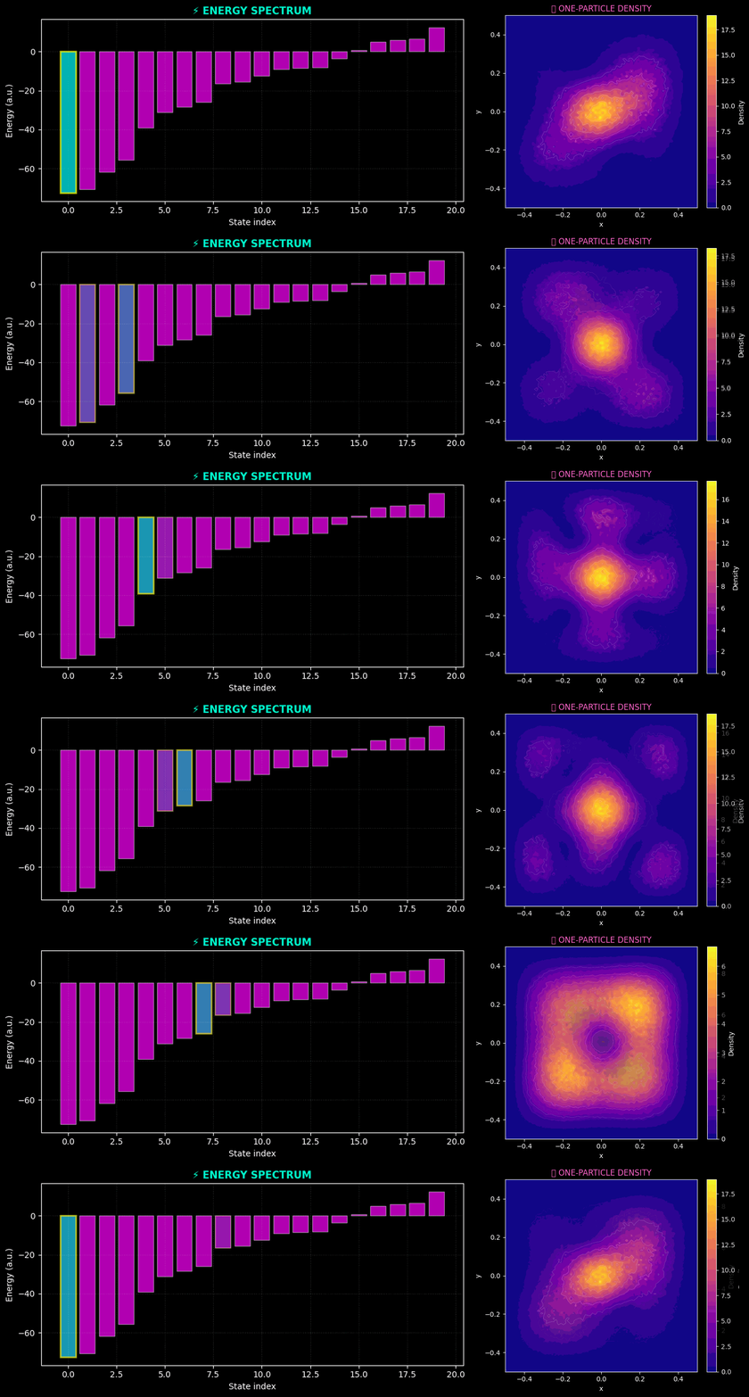 [Two electrons in a well of side L = 1.0 with a carbon nucleus at center and 4 hydrogen nucleus around]
📊 Jupyter Notebook Dashboard (Example Usage, check examples folder)
In a full Jupyter workflow, QOrbit is best experienced as an interactive scientific dashboard where each stage of the quantum simulation is visualized sequentially:
- Initialization of Slater determinant basis
- Construction of Hamiltonian matrix
- Real-time diagonalization profiling
- Ground-state and excited-state energy spectrum visualization
- Wavefunction density and conditional correlation maps
- Potential landscape switching (H₂, hydron, custom potentials)
This structure allows QOrbit to function as a live quantum mechanics exploration environment rather than a static simulator.
🧠 Conclusion
QOrbit demonstrates that complex quantum systems can be approximated using structured Fourier bases and Slater determinant expansions while still preserving physically meaningful energy ordering, spatial localization, and stability trends. Despite stochastic Monte Carlo integration and finite basis truncation, the framework remains numerically stable and consistent across different potential configurations, making it suitable for exploratory quantum simulation and educational visualization.
📚 Citation
If you use or build upon this work, you may cite it as:
@software{qorbit2026,
  author       = {Abhas Kumar Sinha},
  title        = {QOrbit: A Sandbox Quantum Mechanical Simulator},
  year         = {2026},
  url          = {[https://github.com/abhaskumarsinha/qorbit](https://github.com/abhaskumarsinha/QOrbit)},
  version      = {0.1.0},
  note         = {Numerical quantum mechanics framework using approximation and parallelization strategies}
}
References
- Griffiths, David J., and Darrell F. Schroeter. Introduction to quantum mechanics. Cambridge university press, 2018.
Release history Release notifications | RSS feed


Download files
Download the file for your platform. If you're not sure which to choose, learn more about installing packages.
Source Distribution
Built Distribution
Filter files by name, interpreter, ABI, and platform.
If you're not sure about the file name format, learn more about wheel file names.
Copy a direct link to the current filters
File details
Details for the file qorbit-0.1.2.tar.gz.
File metadata
- Download URL: qorbit-0.1.2.tar.gz
- Upload date:
- Size: 32.9 kB
- Tags: Source
- Uploaded using Trusted Publishing? No
- Uploaded via: twine/6.2.0 CPython/3.12.13
File hashes
| Algorithm | Hash digest | |
|---|---|---|
| SHA256 |
15126fc8cd71b78f5aa880de5eead84a71fc3519d4c92c506a246d1301341c45
|
|
| MD5 |
f3d6d4007c8c078abd664111c0c996d4
|
|
| BLAKE2b-256 |
691cc737b2208c737d363d7dd19e8fd4564e717f47de00ad802229216cda8b79
|
File details
Details for the file qorbit-0.1.2-py3-none-any.whl.
File metadata
- Download URL: qorbit-0.1.2-py3-none-any.whl
- Upload date:
- Size: 37.1 kB
- Tags: Python 3
- Uploaded using Trusted Publishing? No
- Uploaded via: twine/6.2.0 CPython/3.12.13
File hashes
| Algorithm | Hash digest | |
|---|---|---|
| SHA256 |
9c208e3a8f4a19e0b2be766f4a54266d7db15e551c3d805123ce1fbb4fc650d6
|
|
| MD5 |
a5a06decace6b34289c446c89b8a488a
|
|
| BLAKE2b-256 |
04cbb23295a00678af0565ccb7854ae35d60270a0c61cfb0778c57c3b8d4adc7
|






