Self Organizing Maps efficient implementation using PyTorch and JAX

Project description
Self-Organizing Map
PyTorch implementation of a Self-Organizing Map. The implementation makes possible the use of a GPU if available for faster computations. It follows the scikit package semantics for training and usage of the model. It also includes runnable scripts to avoid coding.
Example of a MD clustering using quicksom:
Requirements and setup
The SOM object requires PyTorch installed.
It has dependencies in numpy, scipy and scikit-learn and scikit-image. The MD application requires pymol to load the trajectory that is not included in the dependencies
To set up the project, we suggest using conda environments. Install PyTorch and run :
pip install quicksom
SOM object interface
The SOM object can be created using any grid size, with a optional periodic topology. One can also choose optimization parameters such as the number of epochs to train or the batch size
To use it, we include three scripts to :
- fit a SOM
- to optionally build the clusters manually with a gui
- to predict cluster affectations for new data points
$ quicksom_fit -h

usage: quicksom_fit [-h] [-i IN_NAME] [--pdb PDB] [--select SELECT]
                    [--select_align SELECT_ALIGN] [-o OUT_NAME] [-m M] [-n N]
                    [--periodic] [-j] [--n_epoch N_EPOCH]
                    [--batch_size BATCH_SIZE] [--num_workers NUM_WORKERS]
                    [--alpha ALPHA] [--sigma SIGMA] [--scheduler SCHEDULER]

optional arguments:
  -h, --help            show this help message and exit
  -i IN_NAME, --in_name IN_NAME
                        Can be either a .npy file or a .dcd molecular dynamics
                        trajectory. If you are providing a .dcd file, you
                        should also provide a PDB and optional selections.
  --pdb PDB (optional)  If using directly a dcd file, we need to add a PDB for
                        selection
  --select SELECT (optional)
                        Atoms to select
  --select_align SELECT_ALIGN (optional)
                        Atoms to select for structural alignment
  -o OUT_NAME, --out_name OUT_NAME
                        name of pickle to dump
  -m M, --m M           The width of the som
  -n N, --n N           The height of the som
  --periodic            if set, periodic topology is used
  -j, --jax             To use the jax version
  --n_epoch N_EPOCH     The number of iterations
  --batch_size BATCH_SIZE (optional)
                        The batch size to use
  --num_workers NUM_WORKERS (optional)
                        The number of workers to use
  --alpha ALPHA (optional)
                        The initial learning rate
  --sigma SIGMA (optional)
                        The initial sigma for the convolution
  --scheduler SCHEDULER (optional)
                        Which scheduler to use, can be linear, exp or half
You can also use the following two scripts to use your trained SOM.
$ quicksom_gui -h
$ quicksom_predict -h
The SOM object is also importable from python scripts to use directly in your analysis pipelines :
import numpy
from quicksom.som import SOM

# Get data
X = numpy.load('contact_desc.npy')

# Create SOM object and train it, then dump it as a pickle object
m, n = 100, 100
dim = X.shape[1]
n_epoch = 5
batch_size = 100
som = SOM(m, n, dim, n_epoch=n_epoch)
learning_error = som.fit(X, batch_size=batch_size)
som.save_pickle('som.p')

# Usage on the input data, predicted_clusts is an array of length n_samples with clusters affectations
som.load_pickle('som.p')
predicted_clusts, errors = som.predict_cluster(X)
Using JAX
JAX is an efficient array computation library that enables just-in-time (jit) compilation of functions. We recently enabled jax support for our tool. Jax accelerated SOM usage was reported to run twice faster than using the torch backend.
JAX can be installed following these steps. Then the tools usually expose a -j option to use the JAX backend. For instance, try running :
quicksom_fit -i data/2lj5.npy -j
We have kept a common interface for most of the function calls. You should not have to adapt your scripts too much, except for the device management that has a different syntax in JAX. For examples, look at the executable scripts. To use JAX from your scripts, simply change the import in the following manner.
# Classic import, to use the torch backend
from quicksom.som import SOM
# Jax import
from quicksom.somax import SOM
SOM training on molecular dynamics (MD) trajectories
Scripts and extra dependencies:
To deal with trajectories, we use the following new libraries : Pymol, pymol-psico, MDAnalysis. To set up these dependencies using conda, just type :
conda install -c schrodinger pymol pymol-psico
pip install MDAnalysis
Fitting a SOM to an MD trajectory
In MD trajectories, all atoms including solvant can be present, making
the coordinates in each frame unnecessary big and impractical. We offer
the possibility to only keep the relevant indices using a pymol selection,
for instance --select name CA. Moreover, before clustering the conformations,
we need to align them.
Approach 1 : We used to rely on a two step process to fit a SOM to a trajectory :
- Create a npy file with aligned atomic coordinates of C-alpha, using an utility script :
dcd2npy - Fit the SOM as above using this npy file.
Approach 2 : In our new version of the SOM, we skip the intermediary step and rely on PyTorch efficient multiprocess data loading to align the data on the fly. Moreover this approach scales to trajectories that don't fit in memory. It is now the recommended approach.
The two alternative sets of following commands can be applied for a MD clustering :
$ quicksom_fit -i data/2lj5.dcd --pdb data/2lj5.pdb --select 'name CA' -o data/som_2lj5.p --n_iter 100 --batch_size 50 --periodic --alpha 0.5
OR USE THE TWO-STEP PROCESS
$ dcd2npy --pdb data/2lj5.pdb --dcd data/2lj5.dcd --select 'name CA'
$ quicksom_fit -i data/2lj5.npy -o data/som_2lj5.p --n_iter 100 --batch_size 50 --periodic --alpha 0.5

1/100: 50/301 | alpha: 0.500000 | sigma: 25.000000 | error: 397.090729 | time 0.387760
4/100: 150/301 | alpha: 0.483333 | sigma: 24.166667 | error: 8.836357 | time 5.738029
7/100: 250/301 | alpha: 0.466667 | sigma: 23.333333 | error: 8.722509 | time 11.213565
[...]
91/100: 50/301 | alpha: 0.050000 | sigma: 2.500000 | error: 5.658005 | time 137.348755
94/100: 150/301 | alpha: 0.033333 | sigma: 1.666667 | error: 5.373021 | time 142.033695
97/100: 250/301 | alpha: 0.016667 | sigma: 0.833333 | error: 5.855451 | time 147.203326
Analysis and clustering of the map using quicksom_gui:
quicksom_gui -i data/som_2lj5.p
Analysis of MD trajectories with this SOM
We now have a trained SOM and we can use several functionalities such as clustering input data points and grouping them into separate dcd files, creating a dcd with one centroid per fram or plotting of the U-Matrix and its flow.
Cluster assignment of input data points:
quicksom_predict -i data/2lj5.npy -o data/2lj5 -s data/som_2lj5.p
This command generates 3 files:
$ ls data/2lj5_*.txt

data/2lj5_bmus.txt
data/2lj5_clusters.txt
data/2lj5_codebook.txt
containing the data:
- Best Matching Unit with error for each data point - Cluster assignment - Assignment for each SOM cell of the closest
data point (BMU with minimal error).
-1means no assignment
$ head -3 data/2lj5_bmus.txt

38.0000 36.0000 4.9054
37.0000 47.0000 4.6754
2.0000 27.0000 7.0854
$ head -3 data/2lj5_clusters.txt

4 9 22 27 28 32 39 43 44 45 46 48 75 77 78 92 94 98 102 119 126 127 142 147 153 154 162 171 172 180 185 189 190 191 197 206 218 223 226 227 235 245 255 265 285 286 292 299
3 5 7 10 14 21 23 26 29 33 37 51 54 55 63 64 70 74 80 82 83 84 85 86 88 99 103 104 106 107 108 116 121 123 129 131 132 133 139 140 146 148 150 155 159 161 163 165 170 173 179 181 183 200 209 214 217 220 221 228 229 231 237 239 240 241 247 248 250 251 256 258 260 267 275 277 278 279 287 291 293 296 297 301
1 2 8 11 12 13 15 17 18 19 20 24 25 30 31 35 38 41 42 50 52 56 58 60 61 62 65 66 68 69 71 72 73 79 87 89 90 91 93 95 96 97 101 105 109 110 112 113 114 118 120 122 124 125 130 134 136 137 138 141 143 144 145 151 152 156 157 158 160 166 168 169 174 175 176 177 178 184 187 188 193 195 201 205 208 210 211 212 213 215 216 222 225 230 232 233 234 236 242 244 246 249 252 253 254 259 261 262 264 266 268 270 271 272 274 276 280 282 283 284 288 289 290 295 298 300
Cluster extractions from the input dcd using the quicksom_extract tool:
$ quicksom_extract -h

Extract clusters from a dcd file
    quicksom_extract -p pdb_file -t dcd_file -c cluster_file
quicksom_extract -p data/2lj5.pdb -t data/2lj5.dcd -c data/2lj5_clusters.txt
$ ls -v data/cluster_*.dcd

data/cluster_1.dcd
data/cluster_2.dcd
data/cluster_3.dcd
data/cluster_4.dcd
Extraction of the SOM centroids from the input dcd
grep -v "\-1" data/2lj5_codebook.txt > _codebook.txt
mdx --top data/2lj5.pdb --traj data/2lj5.dcd --fframes _codebook.txt --out data/centroids.dcd
rm _codebook.txt
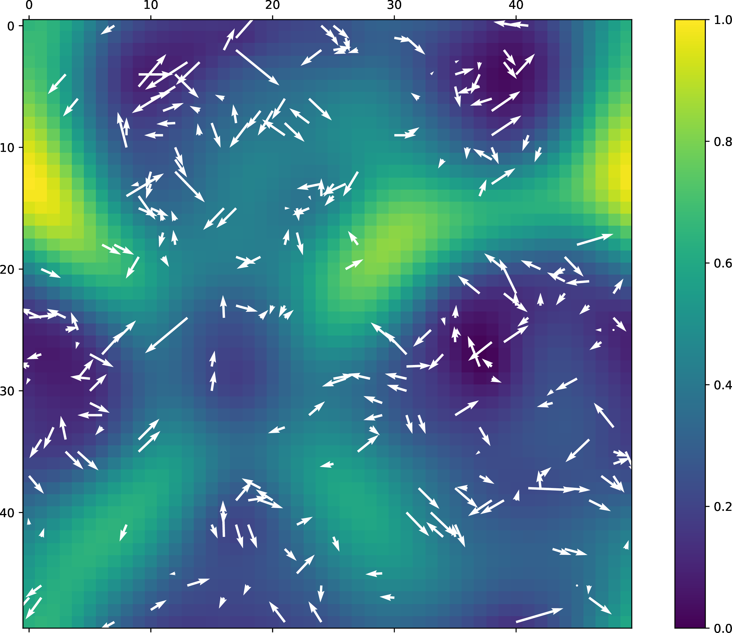
Plotting the U-matrix:
python3 -c 'import pickle
import matplotlib.pyplot as plt
som=pickle.load(open("data/som_2lj5.p", "rb"))
plt.matshow(som.umat)
plt.savefig("data/umat_2lj5.png")
'
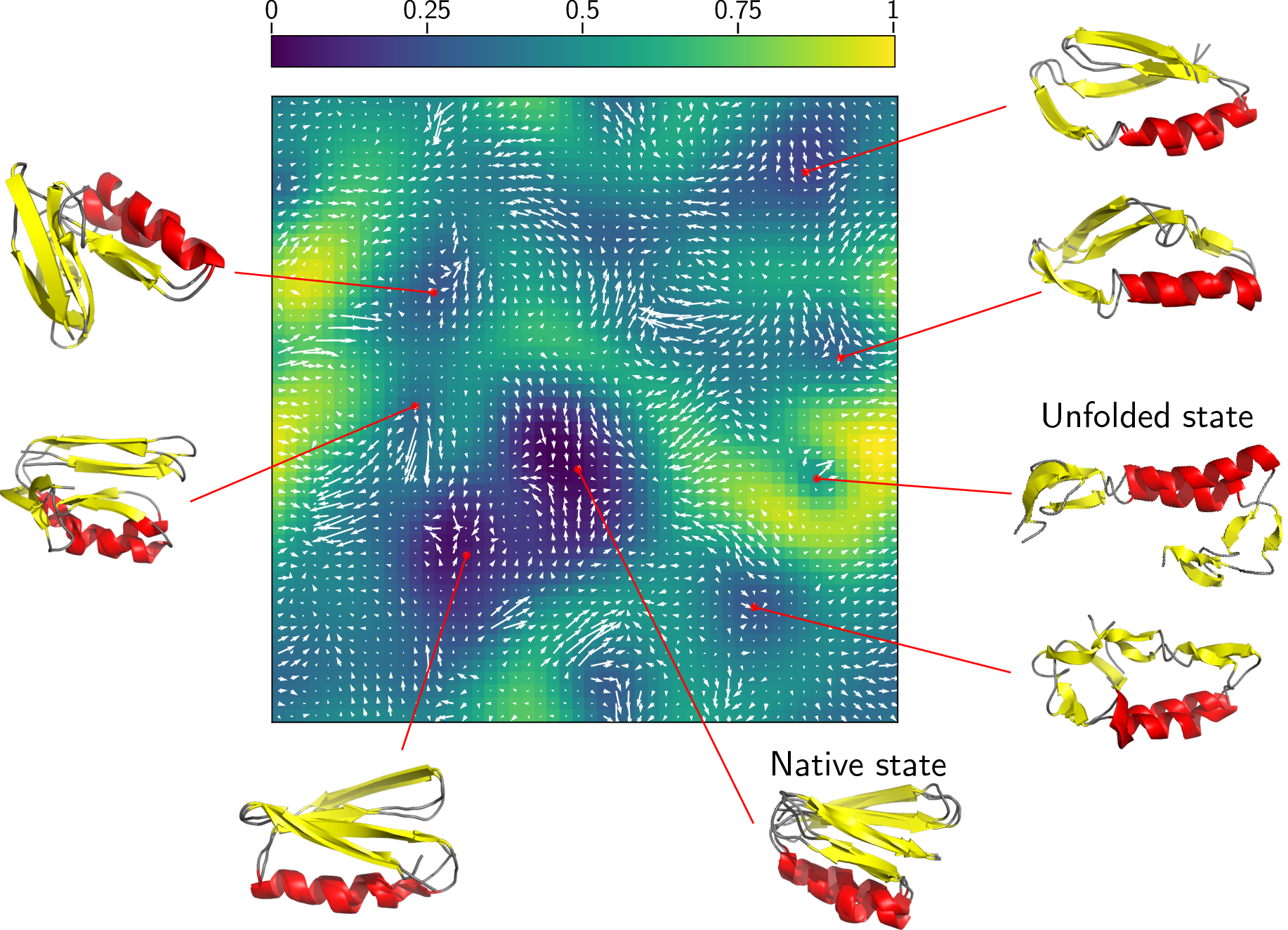
Flow analysis
The flow of the trajectory can be projected onto the U-matrix using the following command:
$ quicksom_flow -h

usage: quicksom_flow [-h] [-s SOM_NAME] [-b BMUS] [-n] [-m] [--stride STRIDE]

Plot flow for time serie clustering.

optional arguments:
  -h, --help            show this help message and exit
  -s SOM_NAME, --som_name SOM_NAME
                        name of the SOM pickle to load
  -b BMUS, --bmus BMUS  BMU file to plot
  -n, --norm            Normalize flow as unit vectors
  -m, --mean            Average the flow by the number of structure per SOM
                        cell
  --stride STRIDE       Stride of the vectors field
With this toy example, we get the following plot:
Data projection
$ quicksom_project -h

usage: quicksom_project [-h] [-s SOM_NAME] [-b BMUS] -d DATA

Plot flow for time serie clustering.

optional arguments:
  -h, --help            show this help message and exit
  -s SOM_NAME, --som_name SOM_NAME
                        name of the SOM pickle to load
  -b BMUS, --bmus BMUS  BMU file to plot
  -d DATA, --data DATA  Data file to project
Miscellaneous
If you run into any bug or would like to ask for a functionnality, feel free to open an issue or reach out by mail.
If this work is of use to you, it was published as an Application Note in Bioinformatics. You can use the following bibtex :
@article{mallet2021quicksom,
  title={quicksom: Self-Organizing Maps on GPUs for clustering of molecular dynamics trajectories},
  author={Mallet, Vincent and Nilges, Michael and Bouvier, Guillaume},
  journal={Bioinformatics},
  volume={37},
  number={14},
  pages={2064--2065},
  year={2021},
  publisher={Oxford University Press}
}


Download files
Download the file for your platform. If you're not sure which to choose, learn more about installing packages.
Source Distribution
Built Distribution
Filter files by name, interpreter, ABI, and platform.
If you're not sure about the file name format, learn more about wheel file names.
Copy a direct link to the current filters
File details
Details for the file quicksom-1.0.0.tar.gz.
File metadata
- Download URL: quicksom-1.0.0.tar.gz
- Upload date:
- Size: 41.6 kB
- Tags: Source
- Uploaded using Trusted Publishing? No
- Uploaded via: twine/3.8.0 pkginfo/1.8.2 readme-renderer/34.0 requests/2.27.1 requests-toolbelt/0.9.1 urllib3/1.26.9 tqdm/4.63.1 importlib-metadata/4.11.3 keyring/23.5.0 rfc3986/2.0.0 colorama/0.4.4 CPython/3.9.11
File hashes
| Algorithm | Hash digest | |
|---|---|---|
| SHA256 |
a1eb00e1b7ba89b4b067ba48dd777af3e6b02ad852bff989c430bc9a807b176d
|
|
| MD5 |
f89c3a2f51ebe9430b2126cba13aeeca
|
|
| BLAKE2b-256 |
db0615901efb11e751be1fc94dabec43d7d38a7f65340b657616ab4368b5f83a
|
File details
Details for the file quicksom-1.0.0-py3-none-any.whl.
File metadata
- Download URL: quicksom-1.0.0-py3-none-any.whl
- Upload date:
- Size: 45.8 kB
- Tags: Python 3
- Uploaded using Trusted Publishing? No
- Uploaded via: twine/3.8.0 pkginfo/1.8.2 readme-renderer/34.0 requests/2.27.1 requests-toolbelt/0.9.1 urllib3/1.26.9 tqdm/4.63.1 importlib-metadata/4.11.3 keyring/23.5.0 rfc3986/2.0.0 colorama/0.4.4 CPython/3.9.11
File hashes
| Algorithm | Hash digest | |
|---|---|---|
| SHA256 |
40b2810eeaf563e08ed47fc111cea569c24cd7ba6ac25837ddd7d88a7afb1fd2
|
|
| MD5 |
e7873af15ed0299d067910bc2bd20e7c
|
|
| BLAKE2b-256 |
21dde8b35defdc1034468a1b7c7e0016222ad0519cec6646a69a13b26c6858b8
|


