
English · 简体中文
realviz — Real Analysis Visualizations
See Riemann and Lebesgue integration side by side. Measure theory for the eyes.



Real analysis is abstract until you see it.
realvizdraws the two great theories of integration on the same function — so the difference finally clicks.
What's the big idea?
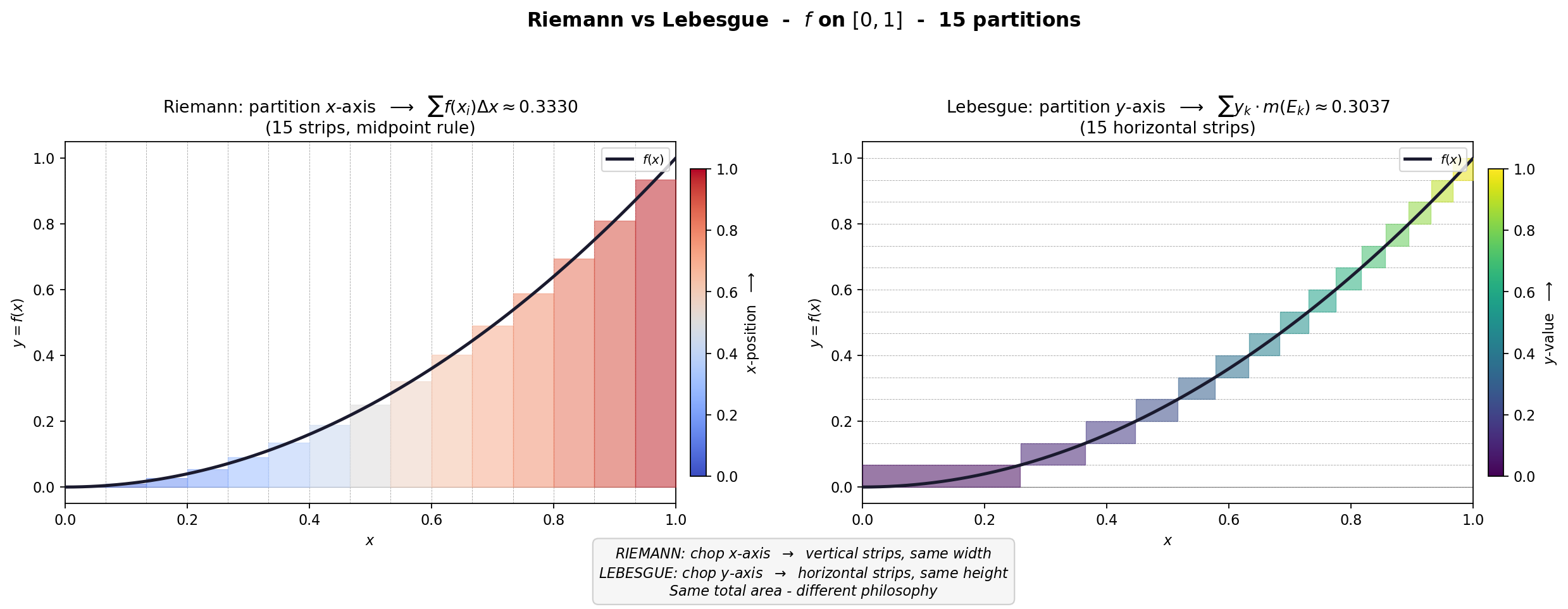
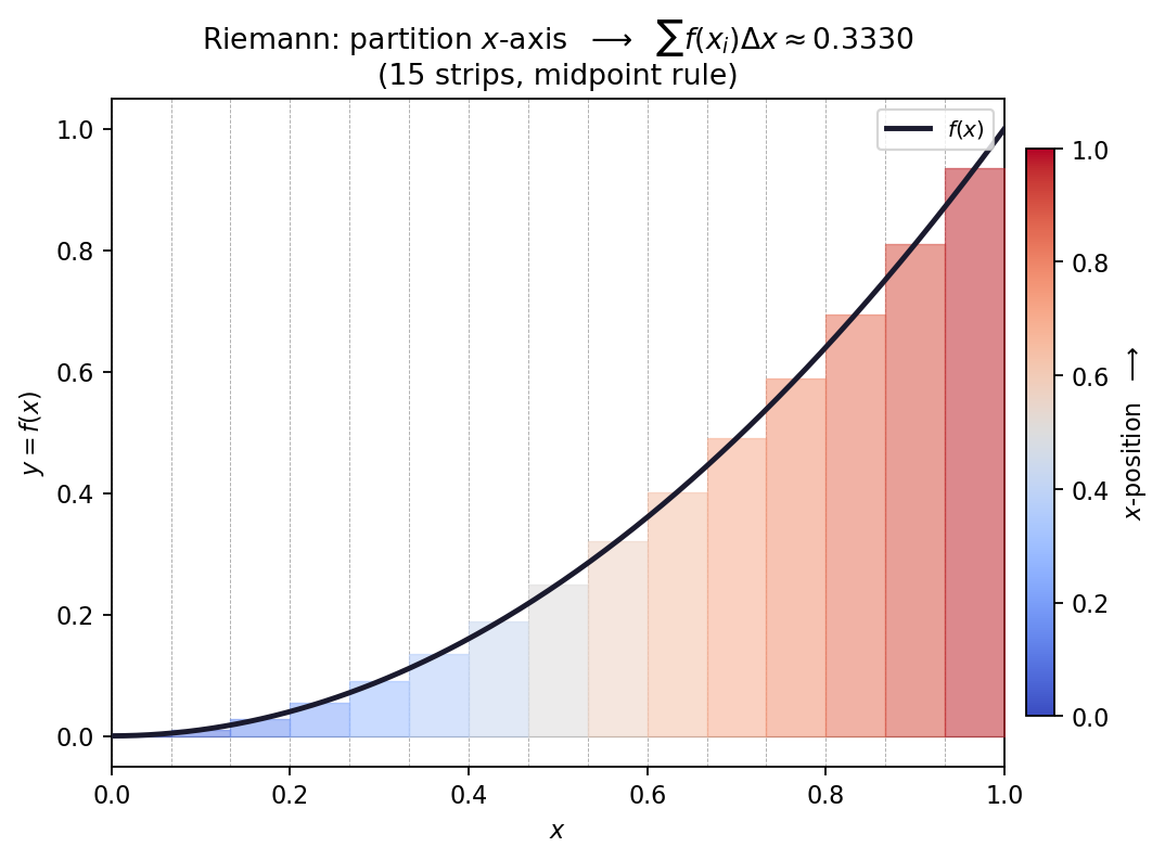
Every calculus student learns Riemann integration first: chop the x-axis into
vertical strips, add up f(xᵢ)·Δx. Lebesgue integration flips it around — chop the
y-axis instead, group points by their function value, and weigh each slice by
the measure of its preimage: Σ yₖ·m(Eₖ).
| Riemann partitions the x-axis | Lebesgue partitions the y-axis |
|---|---|
 |
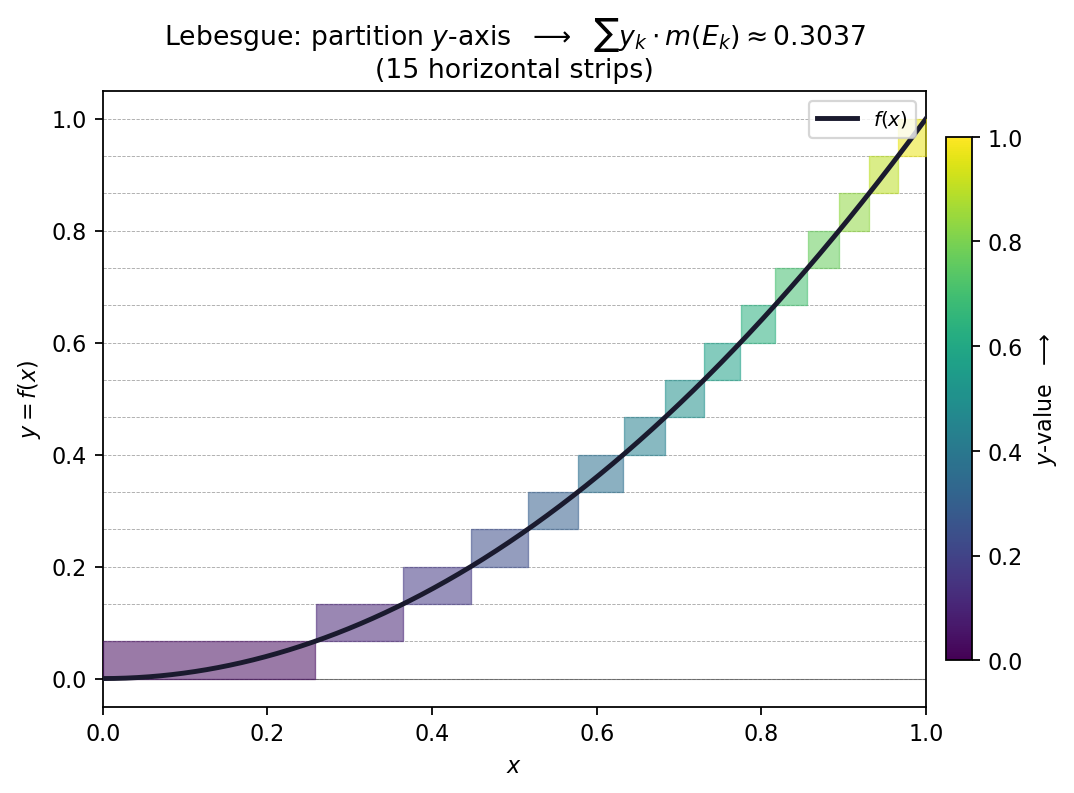 |
| Same-width vertical strips | Same-height horizontal slices |
Sum: Σ f(xᵢ) · Δx |
Sum: Σ yₖ · m(Eₖ) |
| Strip color = x-position | Slice color = y-value |
Same total area. Completely different philosophy.
Where Riemann breaks: the Dirichlet function
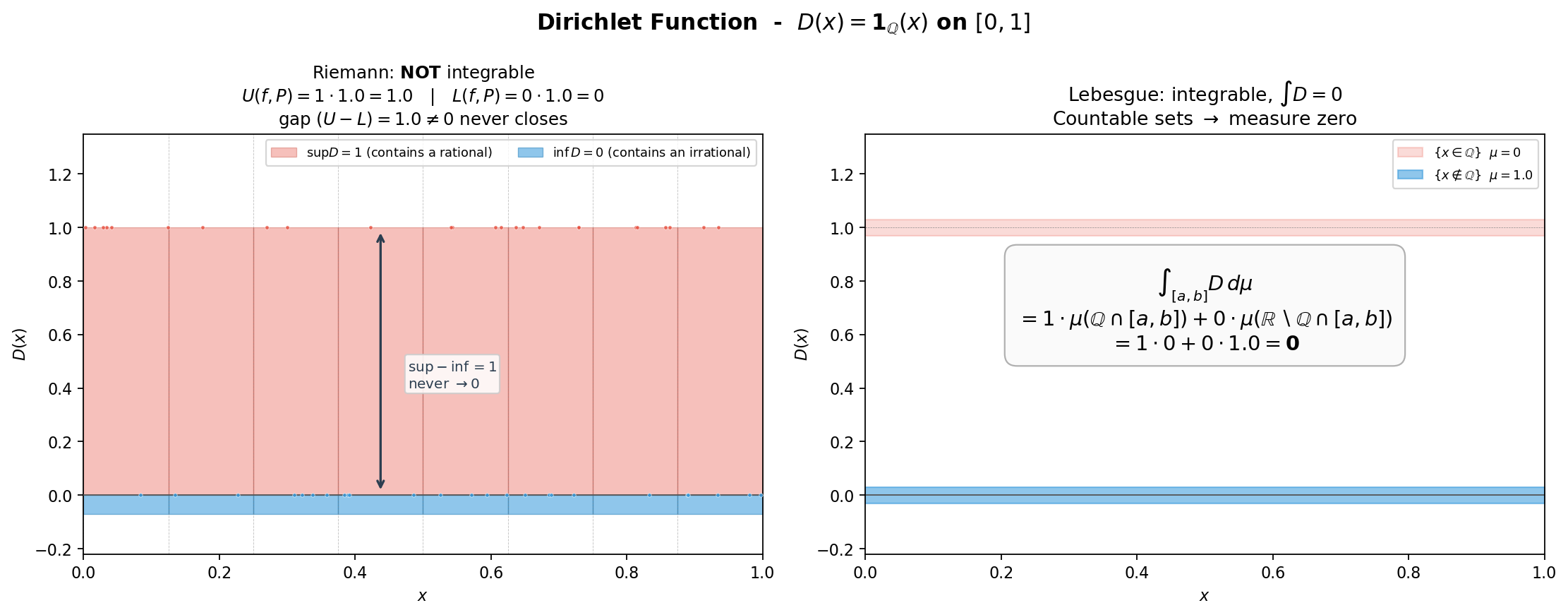
D(x) = 1 if x is rational, 0 otherwise. Every sub-interval of [0,1] contains
both a rational and an irrational — so the upper sum is always 1, the lower sum
always 0, and the gap never closes. Riemann gives up.
Lebesgue measures the irrationals (1) and the rationals (0), and gets a clean
answer: ∫D = 0. This single function motivated a whole field.
Measure zero, yet uncountable: the Cantor set
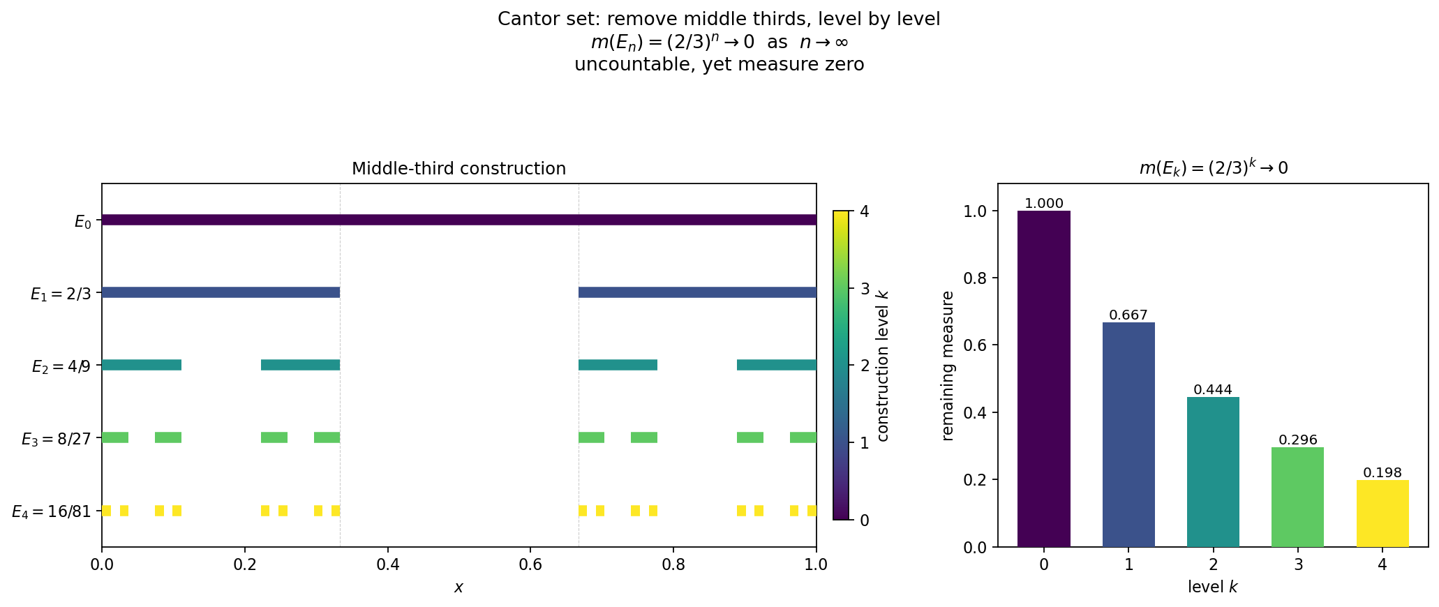
Remove the middle third of [0, 1], then the middle third of every piece that
remains, forever. Row k shows what is left after k removals; the right
panel tracks the surviving measure. m(E_k) = (2/3)^k collapses to 0
exponentially — yet the limiting set has as many points as the real line.
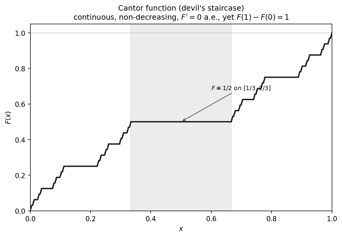
The Cantor function is the staircase this process grows into: continuous,
non-decreasing, flat almost everywhere (F' = 0 a.e.), yet it climbs from 0
to 1 — the counterexample that kills the naive fundamental theorem of calculus.
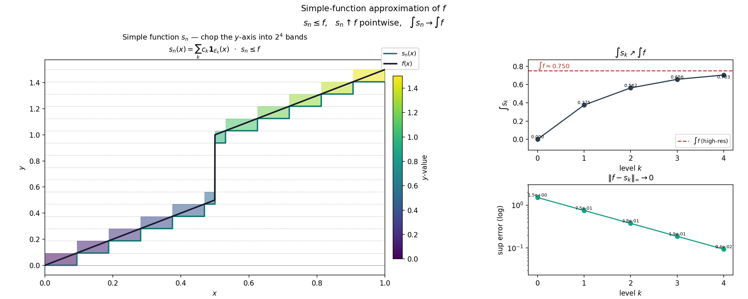
Every measurable function is a limit of simple functions
A simple function takes finitely many values, each constant on a measurable
set. The classic construction cuts the range of f into 2^n equal
horizontal bands and snaps every point down to the lower edge of its band:
sₙ ≤ f, and sₙ climbs to f as n grows. This is the Lebesgue picture
finished — the integral is defined as the limit ∫f = lim ∫sₙ.
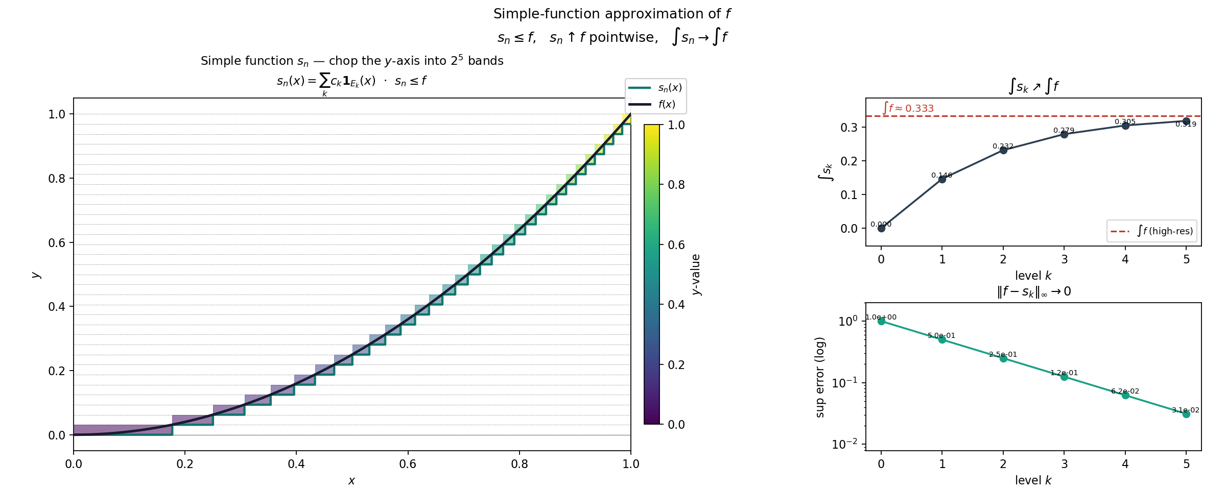
Left: f with sₙ staircased beneath it — each band is a level set
E_k = {x : c_k ≤ f(x) < c_{k+1}}. Top right: ∫s_k rises monotonically to
∫f. Bottom right: the uniform error ‖f − s_k‖∞ → 0 on a log scale.
Simple functions don't care about discontinuities, so oscillations and jumps
are handled just as naturally:
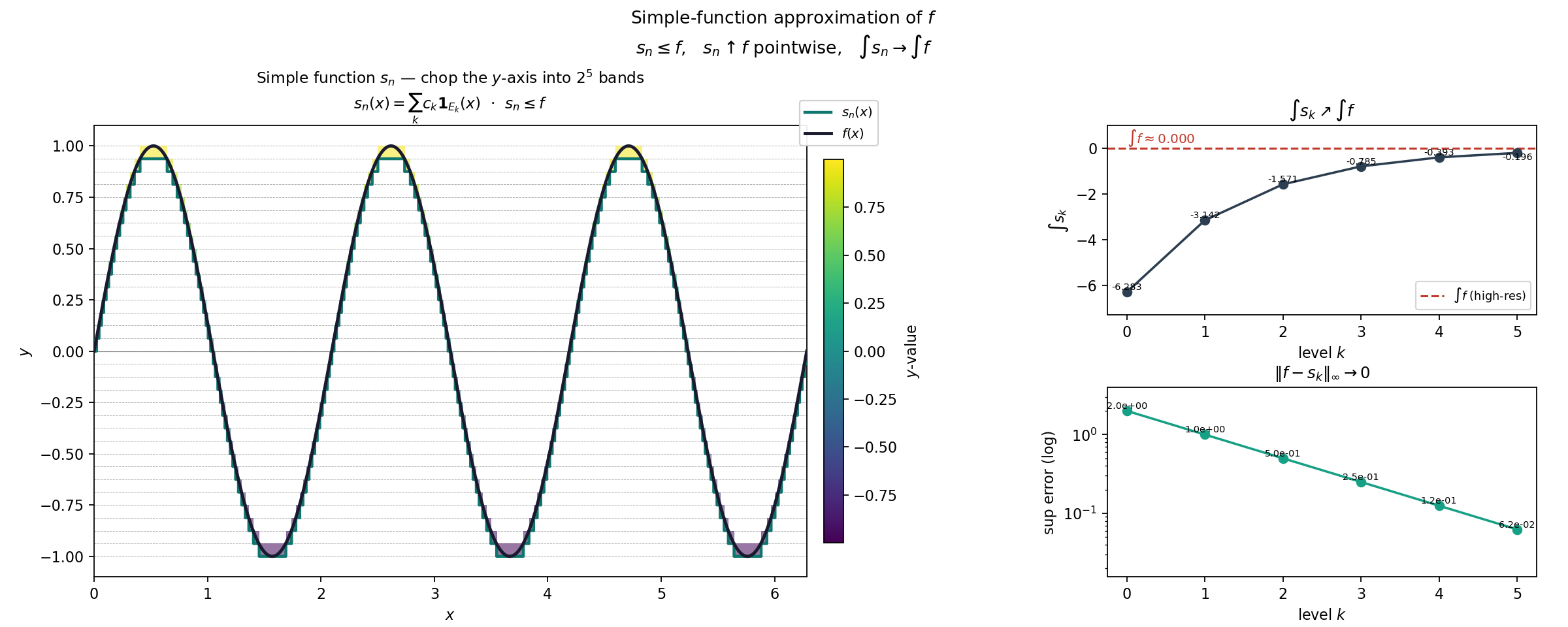
A jump discontinuity changes nothing — the level sets stay measurable, so
∫s_n still converges to the true ∫f = 3/4:
Four ways to converge: one family, four cameras
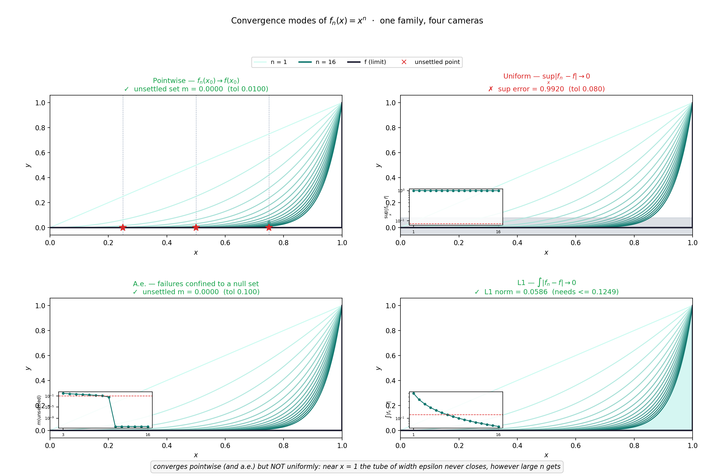
A sequence of functions can converge in genuinely different senses, and the
textbook separates them with three counterexamples. convergence_modes draws
each family once and judges it under four cameras at the same time —
pointwise, uniform, almost-everywhere and L¹ — so the hierarchy breaks apart
in front of you.
The x^n family on [0, 1] converges pointwise and almost everywhere (only
x = 1 is exceptional) and in L¹ — but not uniformly: the ε-tube around
the limit never closes near x = 1.
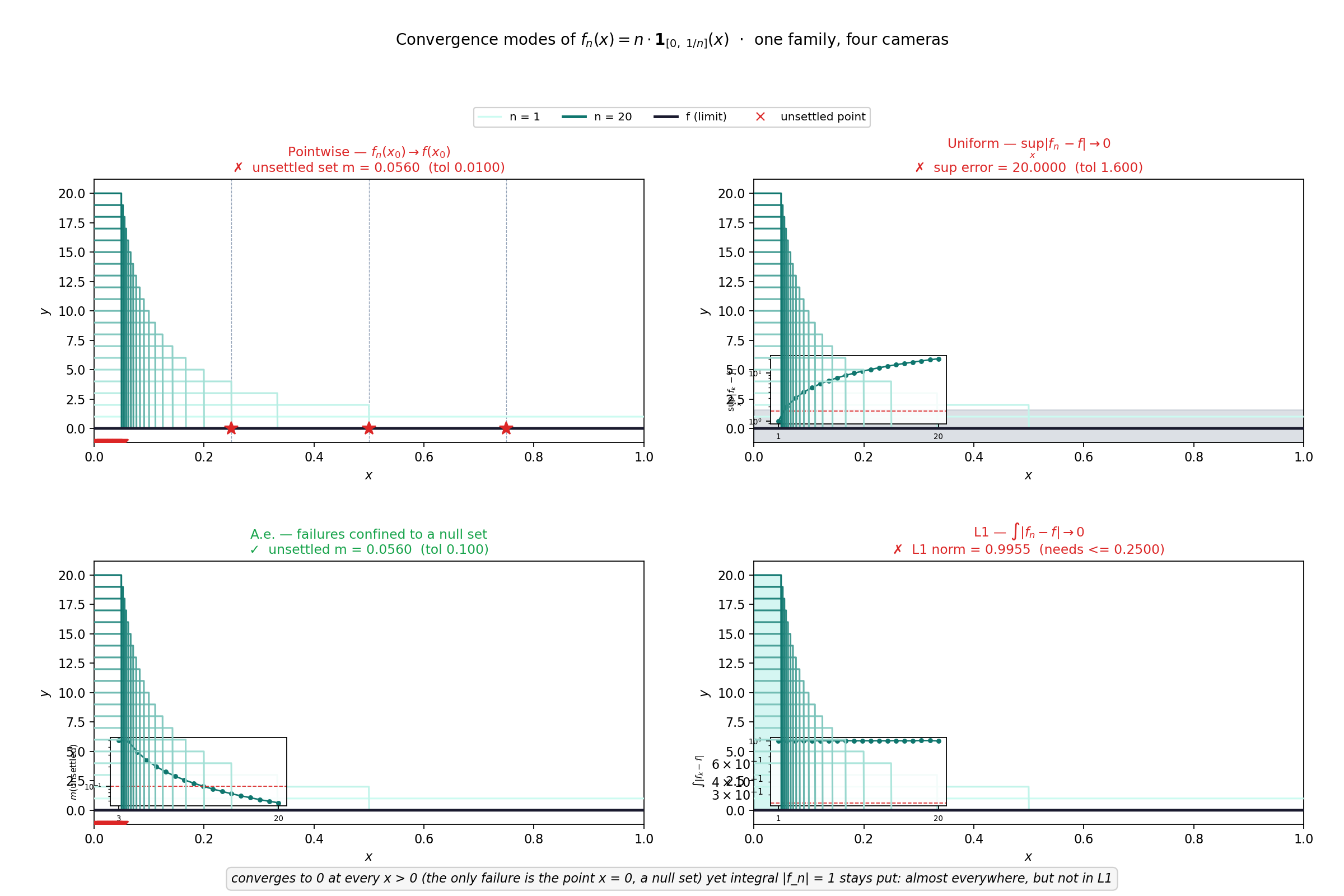
The thin spike n·1_[0, 1/n] collapses onto the single point x = 0 — a null
set — so it converges almost everywhere, yet ∫f_n = 1 stays put:
a.e. but not in L¹.
The typewriter sequence marches an indicator interval across [0, 1], its
width shrinking as it goes. The integrals ∫f_n → 0, so it converges in L¹ —
yet every point is covered infinitely often: it fails at every single point.
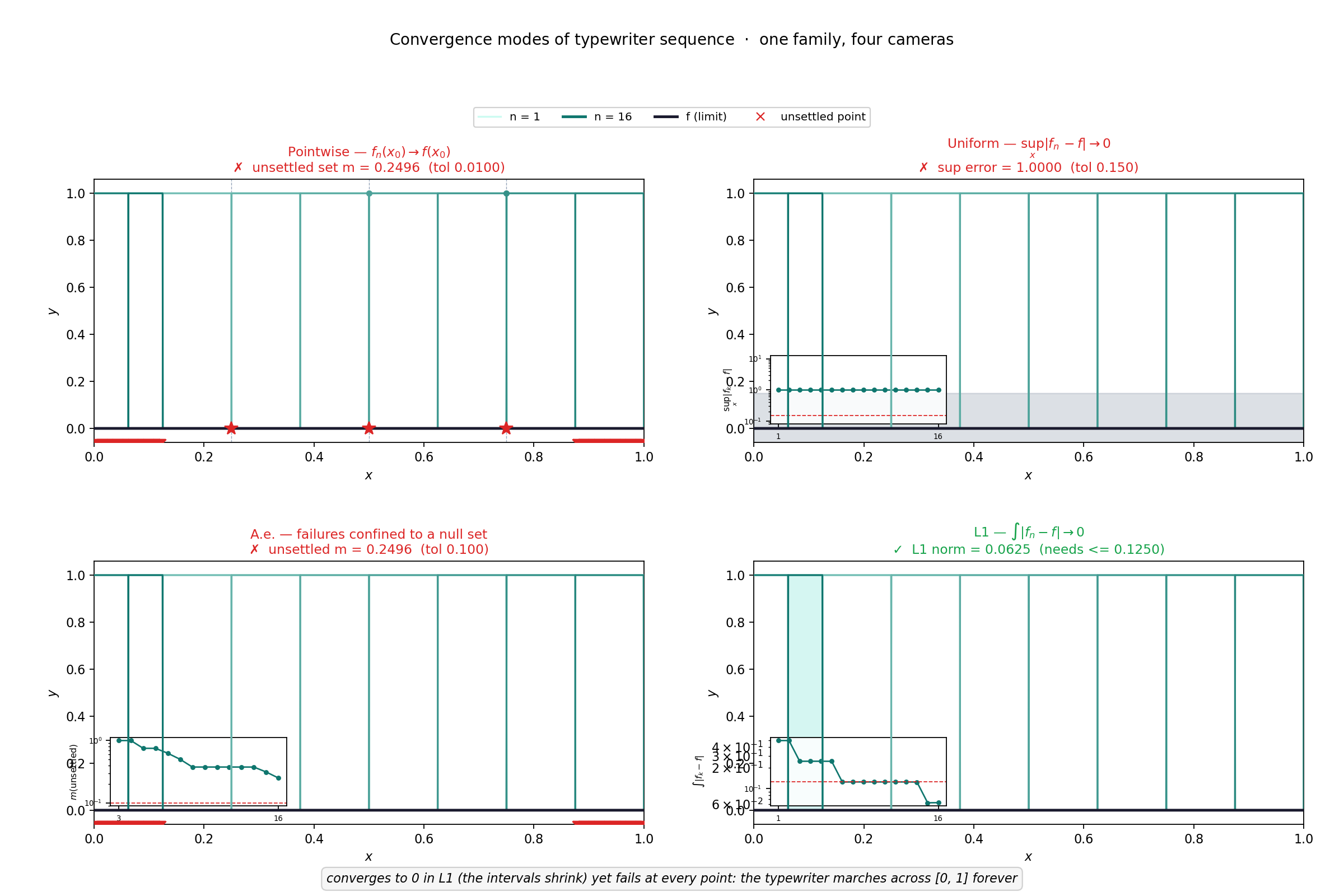
All four panels share one grid, one limit f and one value of ε, and the
verdicts are plain NumPy. Pointwise and a.e. use the same honest finite-window
test — the measure of the set where the last few members still disagree — which
is exactly what separates the spike from the typewriter.
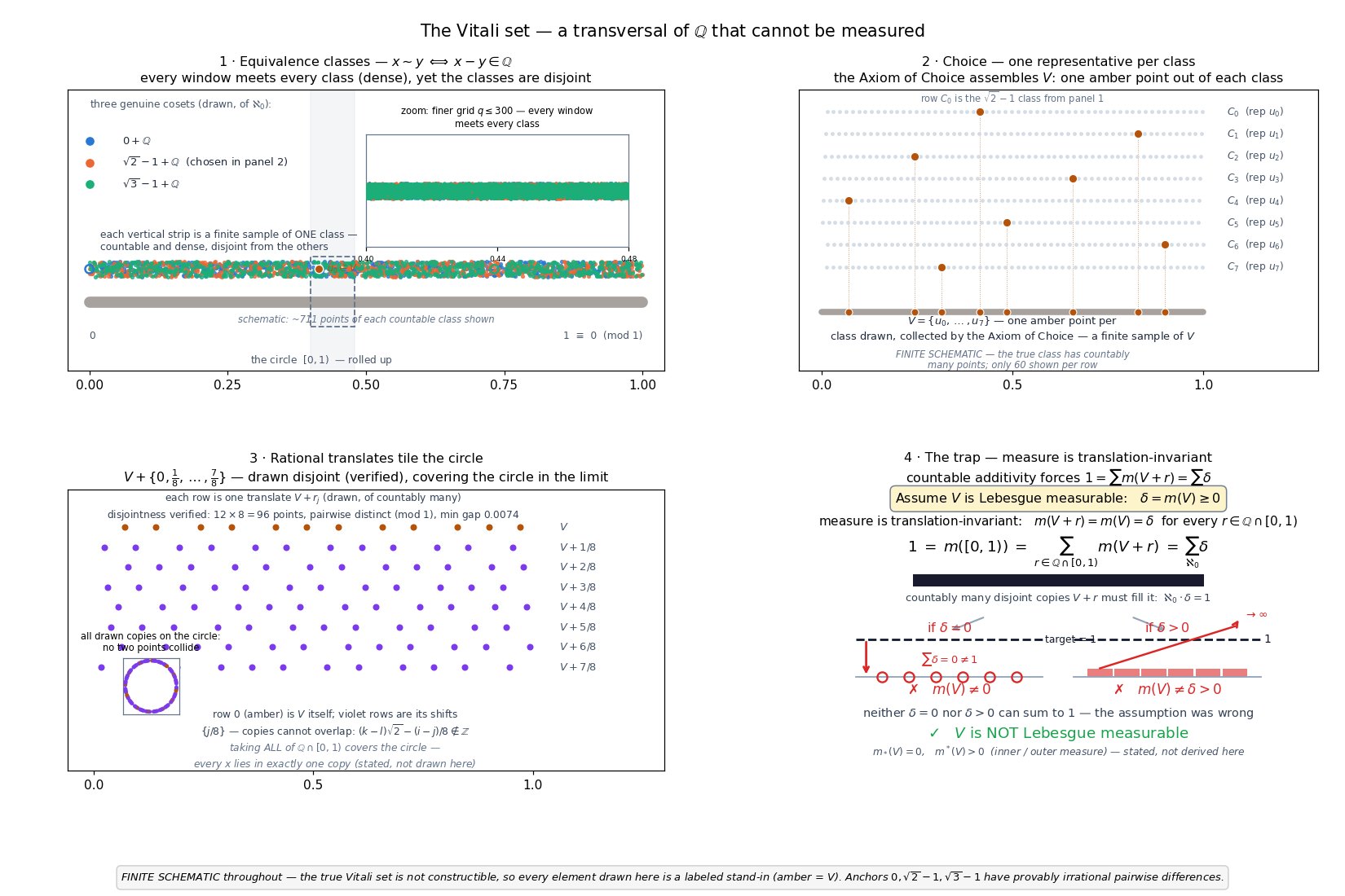
Measure breaks down: the Vitali set
Measure theory's sharpest object is a set that no measure can assign a size
to. Partition the real line into rational cosets x + ℚ — equivalence
classes under x ~ y ⟺ x − y ∈ ℚ, each countable and dense. V is a
transversal: the Axiom of Choice picks one point out of every class.
Shift V by each rational r ∈ ℚ ∩ [0,1). These countably many copies
V + r partition the circle [0,1), so countable additivity demands
1 = m([0,1)) = Σ m(V + r), while translation invariance forces every term to
be the same number m(V) = δ. Hence 1 = Σ_ℵ₀ δ — impossible: the sum is
0 if δ = 0, and infinite if δ > 0. No value of δ works, so V is not
Lebesgue measurable. (Honest, stated not derived: the inner measure is
m_*(V) = 0 and the outer measure satisfies m^*(V) > 0 — it can even be
chosen arbitrarily small, not 1.)
The figure reads as a four-panel proof chain: classes are dense clouds (every
window meets every class), Choice assembles V one point per class, the
translates tile the circle disjointly — verified numerically, 96 points pairwise
distinct mod 1 — and the measure trap snaps shut.
Install
pip install realviz
Quick start
from realviz import compare_integrals, riemann_plot, lebesgue_plot

# Side-by-side comparison — the main event
compare_integrals(lambda x: x**2, 0, 1, n_partitions=15)

# Or inspect each method alone
riemann_plot(lambda x: x**2, 0, 1, n_partitions=10, method="midpoint")
lebesgue_plot(lambda x: x**2, 0, 1, n_partitions=10)

# The Dirichlet function — where Riemann fails, Lebesgue succeeds
from realviz import dirichlet_illustration
dirichlet_illustration()

# The Cantor set and the devil's staircase
from realviz import cantor_set, cantor_function
cantor_set(n_levels=4)     # construction + measure decay
cantor_function()          # F' = 0 a.e., yet F(1) - F(0) = 1

# Simple-function approximation — the Lebesgue story, finished
from realviz import simple_approximation
simple_approximation(lambda x: x**2, 0, 1, n_levels=5)   # s_n -> f, ∫s_n -> ∫f

# Convergence modes — one family, four cameras
from realviz import convergence_modes, FAMILIES
convergence_modes("x_pow_n")     # ✓ pointwise & a.e., ✗ uniform
convergence_modes("thin_spike")  # ✓ a.e., ✗ L1
convergence_modes("typewriter")  # ✓ L1, fails at every point

# The Vitali set — why a transversal of Q has no measure
from realviz import vitali_illustration
vitali_illustration()
Try it yourself
python examples/demo_compare.py     # x² and sin(x), side by side
python examples/demo_dirichlet.py   # the Dirichlet illustration
python examples/demo_cantor.py      # Cantor set + devil's staircase
python examples/demo_simple_approx.py  # simple functions: s_n -> f
python examples/demo_convergence.py    # the three counterexamples, 2x2 grids
python examples/demo_vitali.py         # the Vitali set — a 4-panel proof
Design principles
- Safe by default — strict input validation: functions are sampled defensively,
partition counts are bounded, no
eval/exec/pickle, no network, no file I/O. - Pedagogical color — every strip is colored by what is being partitioned, so the axis-choice is visible at a glance.
- Zero magic — pure NumPy + Matplotlib, ~2,400 lines of core code, MIT licensed.
Roadmap
-
v0.1.0— Riemann vs Lebesgue integral comparison + Dirichlet illustration -
v0.2.0— Cantor set construction + Cantor function (devil's staircase) -
v0.3.0— Simple-function approximation of measurable functions -
v0.4.0— Convergence modes (pointwise, uniform, a.e., in L¹) -
v0.5.0— Vitali set and non-measurable sets (conceptual)
Development
git clone https://github.com/HunterZ549/realviz.git
cd realviz
pip install -e ".[dev]"
pytest               # 230 tests, CI runs Python 3.9–3.12
License
MIT — see LICENSE.
1 maintainer

Metadata
1 maintainer
Release files for realviz 0.5.0
For a detailed explanation of source distributions (sdists) and built distributions (wheels), please see the package formats documentation.
Source distribution (sdist)
| File | Size | Uploaded | |
|---|---|---|---|
| realviz-0.5.0.tar.gz | 2.3 MB | Details |
Built distribution (wheel)
| File | Interpreter | ABI | Platform | Reset |
|---|---|---|---|---|
| realviz-0.5.0-py3-none-any.whl | Python 3 | none | any | Details |
Total release size: 2.4 MB
Release files / realviz-0.5.0.tar.gz
| Download URL | realviz-0.5.0.tar.gz |
|---|---|
| Size | 2.3 MB |
| Tags | Source |
|
SHA-256 checksum How to use checksums |
f80c5df512d7ca7733088861be8896c69d3af8b39892ca0e6bf813cb85a722c5
|
|
BLAKE2b-256 checksum How to use checksums |
1c860f3641aa9d5dd0d40bfd2f2abfc4c00cc5ca78a601fc89f1a40f4d7c0916
|
| Upload date | |
|
Uploaded using Trusted Publishing? What is trusted publishing? |
No |
| Uploaded via |
twine/7.0.0 CPython/3.13.5
|
Release files / realviz-0.5.0-py3-none-any.whl
| Download URL | realviz-0.5.0-py3-none-any.whl |
|---|---|
| Size | 39.0 kB |
| Tags | Python 3 |
|
SHA-256 checksum How to use checksums |
8b2d0b7f39da7d3ee1c1ef8161626d886aac720e77e42c0f6452db7f04887c46
|
|
BLAKE2b-256 checksum How to use checksums |
62c4dcaee137fbc044e0d744f5577bb5caa689b8bcbb281694680a48cf5ed4fa
|
| Upload date | |
|
Uploaded using Trusted Publishing? What is trusted publishing? |
No |
| Uploaded via |
twine/7.0.0 CPython/3.13.5
|














