A fluent time-series and signal processing library for building data pipelines in a single line of Python.

Project description
renkuflow
A clean, chainable Python library for digital signal processing.
renkuflow wraps the power of NumPy and SciPy in a fluent, readable API. Common DSP tasks -
loading audio, filtering, mixing, and spectral analysis - become short, expressive one-liners
instead of 10+ lines of boilerplate.


Example
You can
- Extract data from a .WAV file,
- Apply a bandpass filter on the data,
- Normalise it,
- Take the Fourier transform,
- And plot it.
All in a single line of code!
Signal.from_wav("audio.wav").bandpass(300, 3000).normalize().fft().plot()
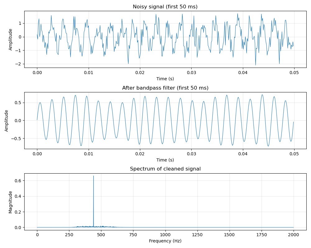
Table of Contents
- Installation
- Core Concepts
- Signal - Constructor Reference
Signal(data, sample_rate)Signal.from_wav(path)Signal.from_audio(path)Signal.from_csv(...)Signal.from_parquet(...)Signal.from_numpy(array, sample_rate, column)Signal.from_pandas(series_or_df, sample_rate, column)Signal.from_matlab(...)Signal.sine(...)Signal.noise(...)Signal.from_function(...)
- Signal - Properties
- Signal - Transformations
- Signal - Filters
- Signal - I/O and Visualization
- Spectrum - Reference
- Worked Examples
- Development
Installation
pip install renkuflow
Install optional extras for the loaders and features you need:
pip install "renkuflow[plot]"    # matplotlib - required for .plot()
pip install "renkuflow[audio]"   # soundfile  - required for Signal.from_audio()
pip install "renkuflow[pandas]"    # pandas + pyarrow - required for from_csv / from_parquet / from_pandas
Combine extras in one command:
pip install "renkuflow[plot,audio,pandas]"
Core requirements: Python 3.11+, NumPy ≥ 1.23.2, SciPy ≥ 1.8
| Extra | Packages installed | Unlocks |
|---|---|---|
plot |
matplotlib | Signal.plot(), Spectrum.plot() |
audio |
soundfile | Signal.from_audio() |
pandas |
pandas, pyarrow | Signal.from_csv(), Signal.from_parquet(), Signal.from_pandas() |
MATLAB files (
.mat) are loaded via SciPy, which is already a core dependency - no extra needed.
Core Concepts
Immutability and chaining
Every transformation returns a new Signal. The original is never modified. This makes it
safe to branch from the same signal and chain operations without side effects:
raw = Signal.from_wav("recording.wav")

# Two independent processing paths from the same source
voice = raw.highpass(80).bandpass(300, 3400).normalize()
full  = raw.lowpass(8000).normalize()
The Signal and Spectrum types
| Type | Domain | Produced by |
|---|---|---|
Signal |
Time (samples × amplitude) | Constructors, transformations |
Spectrum |
Frequency (Hz × magnitude) | Signal.fft() |
Signal - Constructor Reference
Signal(data, sample_rate)
Construct a signal directly from a NumPy array.
import numpy as np
from renkuflow import Signal

data = np.array([0.0, 0.5, 1.0, 0.5, 0.0, -0.5, -1.0, -0.5])
sig = Signal(data, sample_rate=8)
| Parameter | Type | Description |
|---|---|---|
data |
np.ndarray |
1-D array of samples (any numeric dtype, converted to float64 internally) |
sample_rate |
int |
Samples per second (Hz). Must be positive. |
Raises ValueError if data is not 1-D or sample_rate is not positive.
Signal.from_wav(path)
Load a signal from a WAV file.
sig = Signal.from_wav("recording.wav")
- Stereo (or multi-channel) files are averaged to mono.
- Integer PCM samples (e.g. 16-bit) are normalised to the
[-1, 1]range. - Float WAV files are loaded as-is.
| Parameter | Type | Description |
|---|---|---|
path |
str |
Path to the WAV file |
Signal.from_audio(path)
Load a signal from WAV, FLAC, MP3, OGG, and any other audio format supported by the soundfile library.
NOTE: If you are only working with WAV files, using Signal.from_wav(path) is recommended as it doesn't require the soundfile library.
sig = Signal.from_audio("recording.flac")
sig = Signal.from_audio("podcast.mp3")
- Stereo files are averaged to mono.
- Requires the
soundfilepackage (pip install "renkuflow[audio]").
| Parameter | Type | Description |
|---|---|---|
path |
str |
Path to the audio file |
Raises ImportError if soundfile is not installed.
Signal.from_csv(...)
Load a signal from a CSV file.
# Sample rate inferred from a numeric time column
sig = Signal.from_csv("sensor.csv", value_column="voltage", time_column="time_s")

# Sample rate inferred from a datetime column
sig = Signal.from_csv("log.csv", value_column="pressure", time_column="timestamp")

# Explicit sample rate (no time column needed)
sig = Signal.from_csv("raw.csv", value_column="ch0", sample_rate=1000)

# Pass extra pandas kwargs (e.g. delimiter, skip rows)
sig = Signal.from_csv("data.tsv", value_column="amp", time_column="t",
                      sep="\t", skiprows=2)
You must supply either time_column (sample rate is inferred as the median interval) or
an explicit sample_rate. If you supply both, sample_rate wins.
| Parameter | Type | Default | Description |
|---|---|---|---|
path |
str |
- | Path to the CSV file |
value_column |
str |
- | Column containing the signal samples |
time_column |
str | None |
None |
Column with timestamps (numeric seconds or datetime strings) |
sample_rate |
int | None |
None |
Explicit sample rate in Hz |
**pandas_kwargs |
Extra keyword arguments forwarded to pandas.read_csv |
Raises:
ImportError- pandas not installedValueError-value_columnortime_columnnot found in fileValueError- neithertime_columnnorsample_rateprovidedValueError- timestamps are not strictly increasingValueError- fewer than 2 rows (sample rate cannot be inferred)
Signal.from_parquet(...)
Load a signal from a Parquet file. Identical semantics to from_csv.
sig = Signal.from_parquet("sensor.parquet", value_column="voltage", time_column="time_s")

# Explicit sample rate
sig = Signal.from_parquet("data.parquet", value_column="ch0", sample_rate=44100)

# pandas kwargs (e.g. select only needed columns)
sig = Signal.from_parquet("big.parquet", value_column="amp", time_column="t",
                          columns=["t", "amp"])
| Parameter | Type | Default | Description |
|---|---|---|---|
path |
str |
- | Path to the Parquet file |
value_column |
str |
- | Column containing the signal samples |
time_column |
str | None |
None |
Column with timestamps (numeric seconds or datetime strings) |
sample_rate |
int | None |
None |
Explicit sample rate in Hz |
**pandas_kwargs |
Extra keyword arguments forwarded to pandas.read_parquet |
Requires pandas and pyarrow (pip install "renkuflow[pandas]").
Raises the same errors as from_csv plus ImportError if pyarrow is missing.
Signal.from_numpy(array, sample_rate, column)
Load a signal from a NumPy array in memory, or from a .npy / .npz file on disk.
import numpy as np

# From an in-memory array
data = np.random.randn(44100)
sig = Signal.from_numpy(data, sample_rate=44100)

# From a .npy file
sig = Signal.from_numpy("recording.npy", sample_rate=8000)

# From a .npz archive - first array is used automatically
sig = Signal.from_numpy("multi.npz", sample_rate=44100)

# 2-D array (multiple channels) - pick column 1
multichannel = np.random.randn(44100, 4)
sig = Signal.from_numpy(multichannel, sample_rate=44100, column=1)
| Parameter | Type | Default | Description |
|---|---|---|---|
array |
np.ndarray | str |
- | A 1-D or 2-D NumPy array, or a path to a .npy / .npz file |
sample_rate |
int |
- | Samples per second (always required) |
column |
int | None |
None |
Column index to use when array is 2-D |
Raises ValueError if the column index is out of range, the .npz archive is empty, or the
array is not 1-D or 2-D.
Signal.from_pandas(series_or_df, sample_rate, column)
Load a signal from a pandas Series or DataFrame.
import pandas as pd

# From a Series - sample rate inferred from DatetimeIndex
s = pd.Series([0.1, 0.3, -0.2], index=pd.date_range("2024-01-01", periods=3, freq="1ms"))
sig = Signal.from_pandas(s)

# From a Series with a numeric (seconds) index
s = pd.Series([0.1, 0.3, -0.2], index=[0.0, 0.001, 0.002])
sig = Signal.from_pandas(s)

# Explicit sample rate overrides inference
sig = Signal.from_pandas(s, sample_rate=1000)

# From a DataFrame - column name required
df = pd.DataFrame({"ch0": [0.1, 0.3], "ch1": [-0.2, 0.4]})
sig = Signal.from_pandas(df, column="ch0", sample_rate=1000)
Sample rate is inferred automatically when the index is a DatetimeIndex or a numeric index
representing seconds. An explicit sample_rate always takes precedence.
| Parameter | Type | Default | Description |
|---|---|---|---|
series_or_df |
pd.Series | pd.DataFrame |
- | Input data |
sample_rate |
int | None |
None |
Explicit sample rate; inferred from index if omitted |
column |
str | None |
None |
Column name to use when passing a DataFrame (required for DataFrames) |
Raises:
ImportError- pandas not installedTypeError- input is not a Series or DataFrameValueError- DataFrame passed withoutcolumnValueError-columnnot found in DataFrameValueError- fewer than 2 rows (sample rate cannot be inferred)ValueError-sample_ratenot provided and cannot be inferred from the index
Signal.from_matlab(...)
Load a signal from a MATLAB .mat file (supports files up to MATLAB format v7.2).
# Auto-detect the only numeric variable in the file
sig = Signal.from_matlab("recording.mat", sample_rate=44100)

# Name the variable explicitly
sig = Signal.from_matlab("data.mat", variable="ecg", sample_rate=500)

# Read the sample rate from a scalar inside the .mat file
sig = Signal.from_matlab("data.mat", variable="signal", sample_rate_variable="fs")

# Multi-channel array - pick column 2
sig = Signal.from_matlab("eeg.mat", variable="data", sample_rate=256, column=2)
When the file contains exactly one numeric array, variable can be omitted and it is selected
automatically. If sample_rate_variable names a scalar variable in the file (e.g. "fs" or
"Fs"), that value is used; an explicit sample_rate always overrides it.
Note: MATLAB v7.3 files (saved with
-v7.3, which are actually HDF5) are not yet supported. Use an earlier save format from MATLAB if you encounter load errors.
| Parameter | Type | Default | Description |
|---|---|---|---|
path |
str |
- | Path to the .mat file |
variable |
str | None |
None |
Name of the variable to load; auto-selected when there is exactly one numeric array |
sample_rate_variable |
str | None |
None |
Name of a scalar variable in the file that holds the sample rate (e.g. "fs") |
sample_rate |
int | None |
None |
Explicit sample rate; overrides sample_rate_variable |
column |
int | None |
0 |
Column index for multi-channel (2-D) arrays |
Raises ValueError for: missing/ambiguous variable, missing sample rate, column out of range,
or unsupported array shape.
Signal.sine(frequency, duration, sample_rate, amplitude, phase)
Generate a pure sine wave.
# A concert A (440 Hz) for 2 seconds
tone = Signal.sine(frequency=440, duration=2.0)

# Quieter, phase-shifted
tone2 = Signal.sine(frequency=440, duration=2.0, amplitude=0.5, phase=1.57)
| Parameter | Type | Default | Description |
|---|---|---|---|
frequency |
float |
- | Frequency in Hz |
duration |
float |
- | Length in seconds |
sample_rate |
int |
44100 |
Samples per second |
amplitude |
float |
1.0 |
Peak amplitude |
phase |
float |
0.0 |
Phase offset in radians |
Signal.noise(duration, sample_rate, amplitude, seed)
Generate white (Gaussian) noise.
noise = Signal.noise(duration=1.0, amplitude=0.1, seed=42)
| Parameter | Type | Default | Description |
|---|---|---|---|
duration |
float |
- | Length in seconds |
sample_rate |
int |
44100 |
Samples per second |
amplitude |
float |
1.0 |
Standard deviation of the noise |
seed |
int | None |
None |
Random seed for reproducibility |
Signal.from_function(func, duration, sample_rate)
Generate a signal by sampling an arbitrary function of time.
import numpy as np

# Linear chirp sweeping 200 → 1000 Hz over 2 seconds
chirp = Signal.from_function(
    lambda t: np.sin(2 * np.pi * (200 + 400 * t) * t),
    duration=2.0,
    sample_rate=44100,
)

# AM-modulated tone
am = Signal.from_function(
    lambda t: (0.5 + 0.5 * np.sin(2 * np.pi * 2 * t)) * np.sin(2 * np.pi * 440 * t),
    duration=1.0,
)
| Parameter | Type | Default | Description |
|---|---|---|---|
func |
Callable[[np.ndarray], np.ndarray] |
- | Function that accepts a time array t (in seconds) and returns an array of samples |
duration |
float |
- | Length in seconds |
sample_rate |
int |
44100 |
Samples per second |
Signal - Properties
sig.duration
Length of the signal in seconds.
sig = Signal.sine(440, duration=2.5)
print(sig.duration)  # 2.5
sig.sample_rate
Samples per second.
print(sig.sample_rate) # 44100
sig.data
The underlying samples as a np.ndarray of dtype float64.
NOTE: I recommend treating sig.data as read-only.
print(sig.data[:10])
sig.time_axis
NumPy array of the time value (in seconds) for each sample. Useful for plotting.
import matplotlib.pyplot as plt
plt.plot(sig.time_axis, sig.data)
len(sig)
Number of samples.
sig = Signal.sine(440, duration=1.0, sample_rate=8000)
print(len(sig))  # 8000
repr(sig)
Human-readable summary.
print(Signal.sine(440, duration=1.0, sample_rate=8000))
# Signal(samples=8000, sample_rate=8000 Hz, duration=1.000 s)
Signal - Transformations
All transformations return a new Signal. Chains can be as long as needed.
.normalize()
Scale the signal so its peak absolute value is exactly 1.0. Silent signals (all zeros) are returned unchanged.
sig = Signal(np.array([0.0, 0.25, -0.5]), sample_rate=3)
n = sig.normalize()
# n.data → [0.0, 0.5, -1.0]
.trim(start, end)
Extract a time slice. Both arguments are in seconds.
sig = Signal.sine(440, duration=5.0)

# Keep only seconds 1.0 to 3.5
excerpt = sig.trim(start=1.0, end=3.5)
print(excerpt.duration)  # 2.5

# Trim just the start (keep from 0.5 s to end)
trimmed = sig.trim(start=0.5)
| Parameter | Type | Default | Description |
|---|---|---|---|
start |
float |
0.0 |
Start time in seconds |
end |
float | None |
None |
End time in seconds. None means the end of the signal. |
.gain(factor)
Multiply every sample by factor.
sig.gain(2.0)   # double the amplitude
sig.gain(0.5)   # halve the amplitude
.gain_db(db)
Apply gain expressed in decibels. +6 dB ≈ ×2 amplitude; −6 dB ≈ ×0.5 amplitude.
sig.gain_db(6)    # roughly double
sig.gain_db(-20)  # reduce to 10% amplitude
.resample(new_sample_rate)
Change the sample rate. The duration stays the same; the number of samples changes.
# Downsample from 44100 Hz to 8000 Hz (phone quality)
sig_44k = Signal.from_wav("audio.wav")
sig_8k = sig_44k.resample(8000)
sig_a + sig_b - Mixing two signals
Add two signals together (mix them). Both must have the same sample rate. If they have different lengths, the shorter one is zero-padded to match the longer.
tone  = Signal.sine(440, duration=2.0, sample_rate=44100)
noise = Signal.noise(duration=2.0,     sample_rate=44100, amplitude=0.05)
mix   = tone + noise

# Different lengths - result is as long as the longer signal
long_tone   = Signal.sine(440, duration=2.0, sample_rate=44100)
short_noise = Signal.noise(duration=0.5, sample_rate=44100, amplitude=0.1)
mix = long_tone + short_noise  # 2.0 s result
Raises ValueError if the sample rates differ.
Signal - Filters
All filters use a zero-phase Butterworth design (scipy.signal.sosfiltfilt) so they
introduce no time delay. The order parameter controls how sharp the roll-off is -
higher order = steeper but more prone to ringing.
Cutoff frequencies must be strictly between 0 Hz and the Nyquist frequency
(sample_rate / 2). Violating this raises a ValueError.
.lowpass(cutoff, order=4)
Pass frequencies below cutoff, attenuate everything above.
# Remove high-frequency hiss above 4000 Hz
clean = sig.lowpass(cutoff=4000)

# Sharper roll-off
clean = sig.lowpass(cutoff=4000, order=8)
.highpass(cutoff, order=4)
Pass frequencies above cutoff, attenuate everything below.
# Remove low-frequency rumble below 80 Hz
clean = sig.highpass(cutoff=80)
.bandpass(low, high, order=4)
Pass only frequencies between low and high. Everything outside is attenuated.
# Telephone bandwidth: 300–3400 Hz
voice = sig.bandpass(300, 3400)

# Isolate a musical instrument's range
violin = sig.bandpass(196, 3136)
Signal - I/O and Visualization
.to_wav(path)
Save the signal as a 16-bit PCM WAV file. Returns self so it can appear mid-chain.
Values are clipped to [-1, 1] before conversion.
sig.to_wav("output.wav")

# Chain: process then save, then keep working
cleaned = sig.bandpass(300, 3400).normalize().to_wav("cleaned.wav").trim(0.1)
| Parameter | Type | Description |
|---|---|---|
path |
str |
Destination file path |
.plot(title, xlabel, ylabel, ax)
Plot the signal in the time domain using matplotlib. Returns the Axes object.
sig.plot()
sig.plot(title="Raw recording")

# Custom axis labels
sig.plot(xlabel="Time (s)", ylabel="Voltage (V)")

# Embed in an existing figure
fig, axes = plt.subplots(2, 1)
sig.plot(ax=axes[0], title="Before")
filtered.plot(ax=axes[1], title="After")
plt.tight_layout()
plt.show()
| Parameter | Type | Default | Description |
|---|---|---|---|
title |
str | None |
"Signal" |
Plot title |
xlabel |
str | None |
"Time (s)" |
X-axis label |
ylabel |
str | None |
"Amplitude" |
Y-axis label |
ax |
Axes | None |
None |
Existing matplotlib Axes to draw on. Creates a new figure if None. |
.fft()
Convert to the frequency domain. Returns a Spectrum object.
spectrum = sig.fft()
print(spectrum.peak_frequency)  # dominant frequency in Hz
Spectrum - Reference
Spectrum objects are produced by Signal.fft(). They hold paired arrays of frequencies
(Hz) and magnitudes. All magnitudes are normalised so that a sine wave of amplitude 1
has a magnitude of 1 at its frequency.
Properties
| Property | Type | Description |
|---|---|---|
frequencies |
np.ndarray |
Frequency values in Hz for each bin |
magnitudes |
np.ndarray |
Amplitude at each frequency |
peak_frequency |
float |
The frequency with the highest magnitude |
peak_magnitude |
float |
The magnitude at the peak frequency |
len(spec) |
int |
Number of frequency bins |
spec = Signal.sine(440, duration=1.0, sample_rate=8000).fft()

print(spec.peak_frequency)   # 440.0
print(spec.peak_magnitude)   # ≈ 1.0
print(len(spec))             # 4001
print(spec)
# Spectrum(bins=4001, freq_range=(0.0, 4000.0) Hz)
spec.top_n(n=5)
Return the n largest peaks as a list of (frequency, magnitude) tuples, sorted by
magnitude descending.
t = np.arange(8000) / 8000
mixed = np.sin(2 * np.pi * 200 * t) + np.sin(2 * np.pi * 800 * t)
spec = Signal(mixed, sample_rate=8000).fft()

for freq, mag in spec.top_n(2):
    print(f"{freq:.0f} Hz  magnitude={mag:.3f}")
# 200 Hz  magnitude=1.000
# 800 Hz  magnitude=1.000
spec.in_range(low, high)
Return a new Spectrum containing only frequencies in [low, high] Hz.
spec = Signal.from_wav("audio.wav").fft()

# Look at just the sub-bass region
sub_bass = spec.in_range(20, 80)
print(sub_bass.peak_frequency)
spec.plot(title, xlabel, ylabel, log_scale, max_freq, ax)
Plot the magnitude spectrum. Returns the Axes object.
spec.plot()

# Log scale is useful for audio; limit display to 8 kHz
spec.plot(title="Spectrum", log_scale=True, max_freq=8000)

# Custom axis labels
spec.plot(xlabel="Frequency (Hz)", ylabel="Magnitude (linear)")

# Embed in a figure
fig, (ax1, ax2) = plt.subplots(1, 2)
spec.plot(ax=ax1, title="Full spectrum")
spec.in_range(0, 2000).plot(ax=ax2, title="Low frequencies")
plt.show()
| Parameter | Type | Default | Description |
|---|---|---|---|
title |
str | None |
"Frequency Spectrum" |
Plot title |
xlabel |
str | None |
"Frequency (Hz)" |
X-axis label |
ylabel |
str | None |
"Magnitude" |
Y-axis label |
log_scale |
bool |
False |
Use logarithmic Y axis for magnitude |
max_freq |
float | None |
None |
Limit the X axis to this frequency in Hz |
ax |
Axes | None |
None |
Existing Axes to draw on |
Worked Examples
1. Clean a noisy recording
from renkuflow import Signal

noisy = Signal.from_wav("field_recording.wav")

cleaned = (
    noisy
    .highpass(80)           # remove low-frequency rumble
    .bandpass(200, 8000)    # keep speech/music range
    .normalize()
)

cleaned.to_wav("cleaned.wav")
print(f"Peak frequency: {cleaned.fft().peak_frequency:.1f} Hz")
2. Mix signals and analyse the result
from renkuflow import Signal
import numpy as np

sr = 44100
tone_a = Signal.sine(440, duration=2.0, sample_rate=sr)           # A4
tone_b = Signal.sine(554, duration=2.0, sample_rate=sr)           # C#5
tone_c = Signal.sine(659, duration=2.0, sample_rate=sr)           # E5

chord = tone_a + tone_b + tone_c                                  # mix with +
chord = chord.normalize()
chord.to_wav("chord.wav")

# Confirm all three frequencies appear
for freq, mag in chord.fft().top_n(3):
    print(f"{freq:.0f} Hz  (magnitude {mag:.3f})")
# 440 Hz  (magnitude 0.333)
# 554 Hz  (magnitude 0.333)
# 659 Hz  (magnitude 0.333)
3. Plot before and after filtering
import matplotlib.pyplot as plt
from renkuflow import Signal

raw = Signal.from_wav("audio.wav")
filtered = raw.bandpass(300, 3400)

fig, axes = plt.subplots(2, 2, figsize=(14, 6))

raw.trim(0, 0.05).plot(title="Raw (first 50 ms)",      ax=axes[0, 0])
filtered.trim(0, 0.05).plot(title="Filtered (first 50 ms)", ax=axes[0, 1])

raw.fft().plot(title="Raw spectrum",      max_freq=8000, ax=axes[1, 0])
filtered.fft().plot(title="Filtered spectrum", max_freq=8000, ax=axes[1, 1])

plt.tight_layout()
plt.savefig("comparison.png", dpi=120)
4. Load sensor data from a CSV file
from renkuflow import Signal

# CSV with columns: timestamp (ISO 8601), voltage
sig = Signal.from_csv(
    "sensor_log.csv",
    value_column="voltage",
    time_column="timestamp",
)

print(sig)                          # Signal(samples=…, sample_rate=… Hz, duration=… s)
print(sig.fft().peak_frequency)     # dominant frequency in the sensor data

sig.highpass(1).normalize().to_wav("sensor.wav")
5. Load a recording saved from MATLAB
from renkuflow import Signal

# .mat file with variables: 'ecg' (samples) and 'fs' (sample rate scalar)
sig = Signal.from_matlab(
    "ecg_recording.mat",
    variable="ecg",
    sample_rate_variable="fs",
)

print(sig.duration)
sig.bandpass(0.5, 40).plot(title="ECG - bandpass filtered")
6. Load a FLAC file and inspect its spectrum
from renkuflow import Signal

sig = Signal.from_audio("lossless.flac")

spec = sig.fft()
print(f"Peak: {spec.peak_frequency:.1f} Hz @ magnitude {spec.peak_magnitude:.3f}")

spec.plot(title="FLAC spectrum", log_scale=True, max_freq=20000)
Development
If you want to contribute to this project:
- Fork the repository on GitHub,
- Run the following git bash commands to set up an editable clone on your local machine:
git clone https://github.com/yourusername/renkuflow
cd renkuflow
pip install -e ".[dev]"
pytest
- Make a new branch for your edits,
- Make changes,
- Run pytest again to check if anything breaks,
- Commit changes to your fork,
- Open a Pull Request.
License
MIT - © 2026 Sajid Ahmed
Release history Release notifications | RSS feed

Download files
Download the file for your platform. If you're not sure which to choose, learn more about installing packages.
Source Distribution
Built Distribution
Filter files by name, interpreter, ABI, and platform.
If you're not sure about the file name format, learn more about wheel file names.
Copy a direct link to the current filters
File details
Details for the file renkuflow-0.1.1.tar.gz.
File metadata
- Download URL: renkuflow-0.1.1.tar.gz
- Upload date:
- Size: 19.9 kB
- Tags: Source
- Uploaded using Trusted Publishing? No
- Uploaded via: uv/0.11.15 {"installer":{"name":"uv","version":"0.11.15","subcommand":["publish"]},"python":null,"implementation":{"name":null,"version":null},"distro":null,"system":{"name":null,"release":null},"cpu":null,"openssl_version":null,"setuptools_version":null,"rustc_version":null,"ci":null}
File hashes
| Algorithm | Hash digest | |
|---|---|---|
| SHA256 |
001dd5c874348c356df0de93c8f6b2a7903d23d15cb82a358b0f0fd587571d8a
|
|
| MD5 |
14c166232412086e8c25910ecedcc093
|
|
| BLAKE2b-256 |
38087bb476555cc522c24f479337f4eb06522825fc86246675825746383b7e7f
|
File details
Details for the file renkuflow-0.1.1-py3-none-any.whl.
File metadata
- Download URL: renkuflow-0.1.1-py3-none-any.whl
- Upload date:
- Size: 18.2 kB
- Tags: Python 3
- Uploaded using Trusted Publishing? No
- Uploaded via: uv/0.11.15 {"installer":{"name":"uv","version":"0.11.15","subcommand":["publish"]},"python":null,"implementation":{"name":null,"version":null},"distro":null,"system":{"name":null,"release":null},"cpu":null,"openssl_version":null,"setuptools_version":null,"rustc_version":null,"ci":null}
File hashes
| Algorithm | Hash digest | |
|---|---|---|
| SHA256 |
8cb2f33323f838cfda7a5b19bc804689396dcffe13ecaa4eb728e32174475cf9
|
|
| MD5 |
25d65d2bdf836d10814625bfd6ec0261
|
|
| BLAKE2b-256 |
284d5512740f41c66db4905078961c78fb147d6240cbd4bbfcf396f0e0a9c801
|


