Utility functions to assist in the computation of ROC curve comparisons based on academic research.

Project description

Research Utility Package for ROC Curves and AUROC Analysis
Fun Fact: The term “Receiver Operating Characteristic” has its roots in World War II. ROC curves were originally developed by the British as part of the Chain Home radar system. The analysis technique was used to differentiate between enemny aircraft and random noise.
Table of Contents
What are ROC Curves?
What is AUROC analysis?
Hanley and McNeil
Package Overview
- Getting Started
- Find Average Correlation between Two Models
- Find Correlation Coefficient between Two Models
- Q1 and Q2 Calculations
- Get T-Stat to Compare Two Models
- Get Z-Score to Compare Two Models
- Get Non-Parametric AUROC Score
- Get AUROC Bootstrapped P-Value to Compare Two Models
- Create Stacked ROC Plot for Multiple Models
- Get Optimal Classification Threshold from ROC Curve
- Get Optimal Classification Threshold from ROC Curve for Imbalanced Dataset
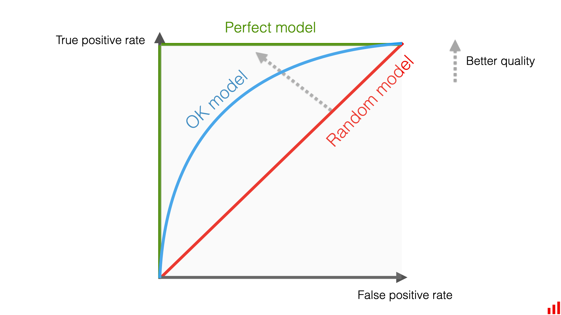
What are ROC Curves?
ROC, or Receiver Operating Characteristic Curve, is essentially a graph that shows how well a binary classification problem is performing. When observing the graph, there is a straight line cutting through the graph at a 45 degree angle. This line represents random guessing, i.e. the model is no better at classifying a class than a coin flip.
$$ \text{Recall} = \frac{\text{True Positives}}{\text{True Positives} + \text{False Negatives}} $$
On the x-axis is the FPR. It is the ratio of false positive predictions to the total number of actual negative instances.
$$ \text{FPR} = \frac{\text{False Positives}}{\text{False Positives} + \text{True Negatives}} $$
The shows the tradeoff between these two metrics at different thresholds for classification. The threshold simply meaning the cutoff point for a positive classification.
$$ f(X, \tau) = \begin{cases} 1 & \text{if } X > \tau \ 0 & \text{otherwise} \end{cases} $$
The way to interpret the graph visually is: the closer the graph's line is to the top left of the plot, the better the model is at making classifications. A perfectly classifying model would go straight from zero up to the top-left corner and then straight across the graph horizontally.
What is AUROC analysis?
While visual inspection of the ROC plot is sufficient in certain cases, oftentimes it can be beneficial to dive deeper in the model's effectiveness. This is where AUROC, or Area Under the Receiver Operating Characteristic, analysis comes into play. It is exactly what it sounds like, in the sense that it is literally the area under the ROC curve. Conceptually, it is a single number which quantifies the overall ability of the model to classify beyond visual inspection alone. It is a score which ranges between 0 and 1, where 0.5 represents random guessing and 1 represents perfect performance. There are several different ways to calculate the AUROC score, but the most common method is to use the trapezoidal rule. This is not something anyone would ever calculate by hand, but the mechanics basically involve forming trapezoids progressively across the graph to estimate the area.
James A. Hanley and Barbara McNeil Methodology
Hanley, of McGill University, and McNeil, of Harvard University, published a landmark paper titled: The Meaning and Use of the Area under a Receiver Operating Characteristic (ROC) Curve in 1982. The duo then followed this paper up in 1983 with another aptly titled landmark paper: A Method of Comparing the Areas under Receiver Operating Characteristic Curves Derived from the Same Cases. To summarize, they created a methodology for using the AUROC score to perform hypothesis tests in order to compare models in a statistically significant way using the Z-Score.
$$ \text{Z} = \frac{AUC_1 - AUC_2}{\sqrt{\frac{V_1 + V_2 - 2 \times \text{Cov}(AUC_1, AUC_2)}{2}}} $$
Hanley and McNeil's methodology has since been adopted and modified by other researchers for applications outside of medicine and is now widely used for analyzing the performance of machine learning models.
ROC Utils Package Methods
This section outlines the methods available with this package. The purpose of these functions is to compare two binary classification models. Whenever a method call for a y_pred parameter, this does NOT refer to the actual predictions of the model, but the probability of a positive classification.
Getting Started
Install and load this package like you would any other pip package.
pip install research-roc-utils
After installation, load in your python file.
import research_roc_utils.roc_utils as ru
Find Average Correlation between Two Models
This function takes y_true, y_pred_1, y_pred_2, and corr_method and returns the average correlation between the positive and negative classifications based on a passed correlation method. IMPORTANT: there is no default correlation method and you must pass in a correlation function. Unless you specifically need this value, it will be called internally by other methods so you will not need to call this method yourself.
import research_roc_utils.roc_utils as ru
from scipy.stats import kendalltau

# avg_corr_fun(y_true, y_pred_1, y_pred_2, corr_method)

avg_corr = ru.avg_corr_fun(y_true, y_pred_1, y_pred_2, kendalltau)
Find Correlation Coefficient between Two Models
This method find the correlation coefficient of two models based on the Hanley and McNeil table. This is commonly represented as r in their papers. The function takes two arguments: the average correlation between the two models for both the positive and negative classifications and the average AUROC between the models. For most methods, you don't need to implement this function yourself and it is called internally.
import research_roc_utils.roc_utils as ru

r_value = ru.avg_corr_fun(avg_corr, avg_area)
Q1 and Q2 Calculations
Unless you specifically need these values individually, you will not need to call this yourself. However, if you want to use these values independently, you can call this method.
import research_roc_utils.roc_utils as ru

from sklearn.metrics import roc_auc_score

roc_auc = roc_auc_score(y_true, y_pred)

q_1, q_2 = ru.q_calculations(roc_auc)
Get T-Stat to Compare Two Models
This method for calculating the T-Stat is adopted from the paper What Predicts U.S. Recessions? (2014) by the researchers Prof. Weiling Liu and Prof. Dr. Emanuel Mönch of Northeastern University and the Frankfurt School of Finance and Management respectively. Their paper is very interesting and I highly recommend reading it if you are interested in learning more about the mechanics and potential application of the ROC T-test. Takes the sklearn roc_auc_score method for calculating AUROC by default. Returns a T-stat which you can use for hypothesis testing.
import research_roc_utils.roc_utils as ru
from scipy.stats import kendalltau

# roc_t_stat(y_true, y_pred_1, y_pred_2, corr_method, roc_auc_fun=roc_auc_score)

t_stat = ru.roc_t_stat(y_true, model_1_y_pred, model_2_y_pred, kendalltau)
Get Z-Score to Compare Two Models
This method is used to calculate the Z-Score based on the implementation of Hanley and McNeil outlined above. This score can be used for hypothesis testing and comparing two models. Also uses the sklearn roc_auc_score as the default roc_auc_fun argument.
import research_roc_utils.roc_utils as ru
from scipy.stats import pearsonr

# roc_z_score(y_true, y_pred_1, y_pred_2, corr_method, roc_auc_fun=roc_auc_score)

z_score = ru.roc_z_score(y_true, y_pred_1, y_pred_2, pearsonr)
Get Non-Parametric AUROC Score
This method is useful in contexts such as econometric or financial analysis when it is not appropriate to assume a specific probability distribution of the data being analyzed. This methodology was adapted from the groundbreaking paper Performance Evaluation of Zero Net-Investment Strategies by Òscar Jordà of the University of California at Davis and Alan M. Taylor also of University of California at Davis. I highly recommend reading their widely cited paper for more information on the theory behind this method.
$$ \text{AUC} = \frac{1}{TN \times TP} \sum_{i=1}^{TN} \sum_{j=1}^{TP} \left( I(v_j < u_i) + \frac{1}{2} I(u_i = v_j) \right) $$
auc = ru.auroc_non_parametric(y_true, y_pred_prob)
Get AUROC Bootstrapped P-Value to Compare Two Models
This method returns a p-value by comparing two models using bootstrapping. The method can be used to perform both one-sided and two-sided hypothesis tests. The structure for the code itself was inspired by another open source project ml-stat-util by @mateuszbuda who is a machine learning researcher based out of Poland. This implementation uses a different methodology for calculating the p-value for two-sided tests, changes the bootstrapping methodology, uses differnt scoring functionality, and is optimized to work with AUROC scores specifically. Returns the p-value as well as a list, l, of the deltas between the two models' AUROC scores based on whatever compare_fun is passed in. Uses the sklearn roc_auc_score as the default score_fun argument.
"""
p, l = boot_p_val(
    y_true,
    y_pred_1,
    y_pred_2,
    compare_fun=np.subtract,
    score_fun=roc_auc_score,
    sample_weight=None,
    n_resamples=5000,
    two_tailed=True,
    seed=None,
    reject_one_class_samples=True
    )
"""

import research_roc_utils.roc_utils as ru

# H0: There is no difference between Model 1 and Model 2
# H1: Model 2 is better than Model 1

p, l = ru.boot_p_val(y_true, model_1_y_pred, model_2_y_pred, n_resamples=10000, two_tailed=False)

if 1 - p < 0.05:
    print("Reject H0 with P-Val of: ", 1 - p)
else:
    print("Insufficient evidence to reject H0")
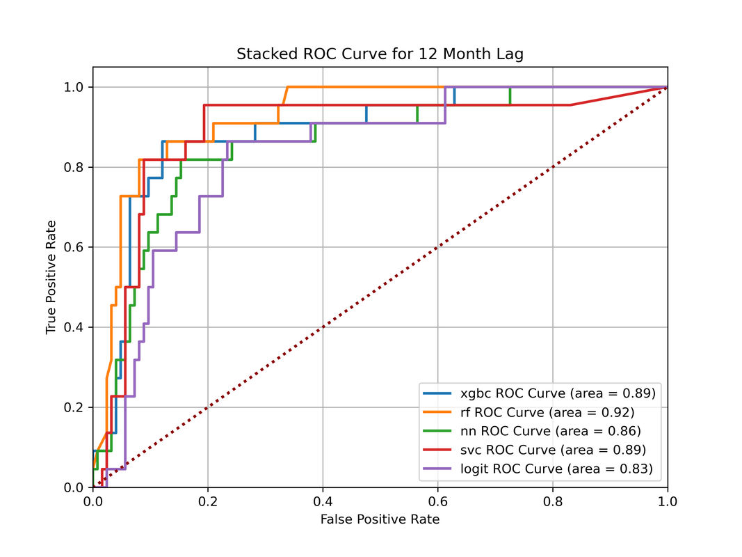
Create Stacked ROC Plot for Multiple Models
This method uses the matplotlib library to easily create a stacked ROC plot of multiple models. Abstracts the functionality for creating the plot itself and returns a plot object with minimal styling which can then be further customized. Uses the sklearn auc method for calculating the AUROC for each model as the default auc_fun. The default roc_fun is from sklearn for generating the TPR and FPR values.
- model_preds: array of prediction probabilities -> list of lists where each item is a model's y_pred values
- model_names: list of strings containing the names for each model in the same order as the model_preds variable
- rand_guess_color: color for the line splitting the plane of the graph representing a random guess
"""
stacked_roc_plt(
        y_true,
        model_preds,
        model_names,
        roc_fun=roc_curve,
        auc_fun=auc,
        fig_size=(8,6),
        linewidth=2,
        linestyle='-',
        rand_guess_color='black'
        )
"""

import research_roc_utils.roc_utils as ru

plt_obj = ru.stacked_roc_plt(y_true, model_preds, model_names, rand_guess_color='darkred')
plt_obj.title("Stacked ROC Curve for 12 Month Lag")
plt_obj.legend(loc="lower right")
plt_obj.grid(True)
plt_obj.show()
Output:
Get Optimal Classification Threshold from ROC Curve
This method returns the optimal threshold based on the ROC curve based on the TPR and FPR. It works by finding the threshold where the delta between the FPR and TPR is maximized.
import research_roc_utils.roc_utils as ru

threshold = ru.optimal_threshold(y_true, y_pred)
Get Optimal Classification Threshold from ROC Curve for Imbalanced Dataset
This method returns the optimal threshold based on the ROC curve, but is optimized for imbalanced datasets. This method uses the geometric mean for finding the best threshold. Check out this link for more details on the implementation:
import research_roc_utils.roc_utils as ru

threshold = ru.optimal_threshold_imbalanced(y_true, y_pred)
Release history Release notifications | RSS feed


Download files
Download the file for your platform. If you're not sure which to choose, learn more about installing packages.
Source Distribution
Built Distribution
Filter files by name, interpreter, ABI, and platform.
If you're not sure about the file name format, learn more about wheel file names.
Copy a direct link to the current filters
File details
Details for the file research_roc_utils-0.1.1.tar.gz.
File metadata
- Download URL: research_roc_utils-0.1.1.tar.gz
- Upload date:
- Size: 18.2 kB
- Tags: Source
- Uploaded using Trusted Publishing? No
- Uploaded via: twine/5.0.0 CPython/3.11.7
File hashes
| Algorithm | Hash digest | |
|---|---|---|
| SHA256 |
04396008da5f6a8d5934d4cadc98ea00fe46b90d3f39a26e1e90eb8f69f2639e
|
|
| MD5 |
78b8bd06b12e963f9cc9ae93508d5328
|
|
| BLAKE2b-256 |
3b6da5d6b03c97ff56c2907423b054a0b1cd44e142ef42efc49be851602a584a
|
File details
Details for the file research_roc_utils-0.1.1-py3-none-any.whl.
File metadata
- Download URL: research_roc_utils-0.1.1-py3-none-any.whl
- Upload date:
- Size: 13.8 kB
- Tags: Python 3
- Uploaded using Trusted Publishing? No
- Uploaded via: twine/5.0.0 CPython/3.11.7
File hashes
| Algorithm | Hash digest | |
|---|---|---|
| SHA256 |
e0d1cc38ea313f965a3144dcbfc79ba40b3c71dd3108b3cc136c9e5fe1a7225b
|
|
| MD5 |
b422c15cdb0142b917e6654ca8d756d7
|
|
| BLAKE2b-256 |
de19807cf942186c5058baf6c2fd00a4ce41dba51a0d4944729b1da14cf1602f
|


