Explore and visualize resilience metrics and antifragility in performance graphs of self-adaptive systems.
Verified details
These details have been verified by PyPIProject links
GitHub Statistics
Maintainers

Project description
ResMetric


ResMetric is a Python module designed to enhance Plotly figures
with resilience-related metrics. This comes in handy if you want
to explore different metrics and choose the best for your project.
The resilience of a system is especially of interest within the field of self-adaptive systems where it measures the adaptability to shocks. But there is still no standard metric.
This package enables users to add various optional traces and analyzes to
Plotly plots to visualize and analyze data more effectively. Therefore,
different resilience metrics can be explored. In addition,
the metrics submodule provides functions that can calculate the metrics individually!
Links
- 🐍 PyPI: pypi.org/project/resmetric/
- 🛠 GitHub Repository: github.com/ferdinand-koenig/resmetric
- 🧾 Artefact / Code DOI: doi.org/10.5281/zenodo.14724651
- 📄 arXiv Preprint: arXiv:2501.18245
- 📘 SEAMS Proceedings: to be published
Please cite both the associated paper and the artefact when using ResMetric. The relevant BibTeX entries can be
found in the appendix of this README.
Key Features
- Separation of Dip-Agnostic ([T-Ag]) and Dip-Dependent Metrics ([T-Dip]): Analyze your performance graph w.r.t. resilience and 'antifragility' (See Getting Started Section)
- Dip-Agnostic Metrics do not depend on where a disruption starts and the system is fully recovered. (AUC, count and time below a threshold, etc)
- Dip-Dependent Metrics need the definition/detection of where a disruption starts and when it is recovered. (AUC per dip, robustness, recovery, recovery rate, Integrated Resilience Metric)
- Customizable Metrics: Adjust parameters for AUC calculations, smoothing functions, and use Bayesian optimization to fit linear regressions to detect steady states and therefore dips. (Advanced)
- Use as Module or CLI: Include the module in one of your projects or use the CLI to interact with the module!
- Display or Save: Display the plot in your browser or save it as an HTML file.
Installation and Setup
The following guide is for beginners. If you are not a beginner, feel free to skip the installation instructions!
If you need the wheel file, you can find it in the releases section of the official repository on GitHub. This is generally not required as the wheel is available via the standard Python distribution: ResMetric on PyPi.
Having trouble installing it? Please check the installation note in the appendix of this README.
Step-by-Step Installation and Setup
Go to a folder where you want to place the installation.
-
Get Python (Only if you do not have Python
>= 3.8)You should download and install Python from download. Go for the latest version, but everything
>= 3.8will be fine. A guide for installation and version check can be found here. -
Install the package Create a virtual environment and install the package in it:
- Linux or MacOS:
python3 -m venv .venv
source .venv/bin/activate
python3 -m pip install --upgrade pip
python3 -m pip install resmetric
- Windows:
py -m venv .venv
.venv\Scripts\activate
py -m pip install --upgrade pip
py -m pip install resmetric
On Windows, the installation takes a few minutes, while on Linux and macOS, it completes in under 30 seconds.
- Linux or MacOS:
-
Use the package If you continue right after step 1, you can use the tool and jump right in. If you have installed the package previously, you have to source your shell again:
-
For Linux or MacOS:
source .venv/bin/activate
-
For Windows:
.venv\Scripts\activate
Now, explore the tool on your own! You can try using the CLI, the module in Python, or check out our CLI Examples to see demonstrations and replicate them.
-
-
After Use To deactivate the virtual environment, run
deactivate
-
Uninstall If you have created the virtual environment only for this project (as you did if you followed this little guide), just delete the
.venvdirectory. That's it!rm -r .venv
You could also uninstall Python if you no longer need it.
Getting started
Familiarize yourself with the workflow. It will help to understand how the dip-agnostic track and dip-dependent track differ and how to calculate 'antifragility' (resilience over time)
resmetric-cli --workflow
Then, try the examples (below).
Module Usage
Importing the Module
To use the ResMetric module, import the create_plot_from_data function from the plot module:
from resmetric.plot import create_plot_from_data
# or
import resmetric.plot as rp
# rp.create_plot_from_data(...)
Using the Function
The create_plot_from_data function generates a Plotly figure from JSON-encoded data and adds optional traces and
analyses.
Function Signature
def create_plot_from_data(json_str, **kwargs):
    """
    Generate a Plotly figure from JSON-encoded data with optional traces and analyses.

    Parameters:
    - json_str (str): JSON string containing the figure data.
    - **kwargs: Optional keyword arguments to include or exclude specific traces and analyses.

    Returns:
    - fig: Plotly Figure object with the specified traces and analyses included.
    """
Optional Keyword Arguments
Preprocessing
include_smooth_criminals(bool): Include smoothed series (seesmoother_threshold).
[T-Ag] Dip-Agnostic Resilience Trace Options
include_auc(bool): Include AUC-related traces. (AUC divided by the length of the time frame and different kernels applied)include_count_below_thresh(bool): Include traces that count dips below the threshold.include_time_below_thresh(bool): Include traces that accumulate time below the threshold.threshold(float): Threshold for count and time traces (default: 80).include_dips(bool): Include detected dips.include_draw_downs_traces(bool): Include traces representing the relative loss at each point in the time series, calculated as the difference between the current value and the highest value reached up to that point, divided by that highest value.include_draw_downs_shapes(bool): Include shapes of local draw-downs.include_derivatives(bool): Include derivatives traces.
[T-Dip] Dip-Dependent Resilience Trace Options
-
dip_detection_algorithm(str): Specifies the dip detection algorithm to use. It can be 'max_dips' (default), 'threshold_dips', 'manual_dips', 'lin_reg_dips' (the last requiresinclude_lin_reg) -
manual_dips(list of tuplesorNone): If 'manual_dips' is selected as the dip detection algorithm, this should be a list of tuples specifying the manual dips. (E.g.,[(2,5), (33,42)]for two dips from time t=2 to 5 and 33 to 42 -
include_lin_reg(boolorfloat): Include linear regression traces. Optionally float for threshold of slope. Slopes above the absolute value are discarded. The threshold defaults to 0.5% (for value set to True). It is possible to passmath.inf. See alsono_lin_reg_prepro -
no_lin_reg_prepro(bool):include_lin_regautomatically preprocesses and updates the series. If you do not wish this, set this flag to True -
include_max_dip_auc(bool): Include AUC bars for the AUC of one maximal dip (AUC devided by the length of the time frame) -
include_bars(bool): Include bars for MDD and recovery. -
include_irm(bool): Include the Integrated Resilience Metric (cf. Sansavini, https://doi.org/10.1007/978-94-024-1123-2_6, Chapter 6, formula 6.12). Requires kwargrecovery_algorithm='recovery_ability'. -
recovery_algorithm(strorNone): Decides the recovery algorithm. Can either beadaptive_capacity(default) orrecovery_ability. The first one is the ratio of new to prior steady state's value(Q(t_ns) / Q(t_0)). The last one isabs((Q(t_ns) - Q(t_r))/ (Q(t_0) - Q(t_r)))whereQ(t_r)is the local minimum within a dip (Robustness). -
calc_res_over_time(bool): Calculate the differential quotient for every per-dip Resilience-Related Trace.
Bayesian Optimization (Only for include_lin_reg)
penalty_factor(float): Penalty factor to penalize many segments / high number of linear regression lines (default: 0.05).dimensions(int): Maximal number of segments for linear regression (default: 10).
AUC-related Options (Only for include_auc)
weighted_auc_half_life(float): Half-life for weighted AUC calculation (default: 2).
Smoothing Function Options (Only for include_smooth_criminals)
smoother_threshold(float): Threshold for the smoothing function in %. If a new point deviates only this much, the old value is preserved / copied (default: 2[%]).
CLI Interface
The module also includes a command-line interface for quick usage.
Command-Line Usage
resmetric-cli [options] json_file
The arguments are similar to the already described ones. For more, see the help page:
resmetric-cli -h
Examples
Use as module
import plotly.graph_objects as go
import resmetric.plot as rp

# Step 1: Create a Plotly figure
fig = go.Figure()  # Example: create a basic figure

# Customize the figure (e.g., add traces, update layout)
# Here you add the data of the performance graph where you want to investigate resilience (over time)
fig.add_trace(go.Scatter(x=[0, 1, 2], y=[.4, .5, .6], mode='lines+markers', name='Q1'))
fig.add_trace(go.Scatter(x=[0, 1, 2], y=[.4, .3, .6], mode='lines+markers', name='Q2'))

# Get the JSON representation of the figure
json_data = fig.to_json()

# Step 2: Generate the plot with additional traces using the JSON data
rp.set_verbose(False)  # disable prints (only relevant for lin reg)
fig = rp.create_plot_from_data(
    json_data,
    include_count_below_thresh=True,
    include_maximal_dips=True,
    include_bars=True
)

# Display the plot
# fig.show()
# There is a bug with fig.show with which in approx. 10% of the cases the webpage would not load
# Since some calculation may take long, the following approach is used with which the problem
# seems to be solved.
fig.write_html('output.html', auto_open=True)

# Save the updated plot as HTML
fig.write_html('plot.html')

print("Figure saved as 'plot.html'")
Use as CLI tool
Note: The wheel (.whl) does not include example material.
To get started, you can download the example data fig.json here.
Please place the downloaded file in a subdirectory called example to use the examples as provided.
For using your own data, create a Plotly plot as in the module example above and usefig.write_json('plot.json').
Do not use the json package for serialization, as Plotly will not be able to deserialize the file correctly.
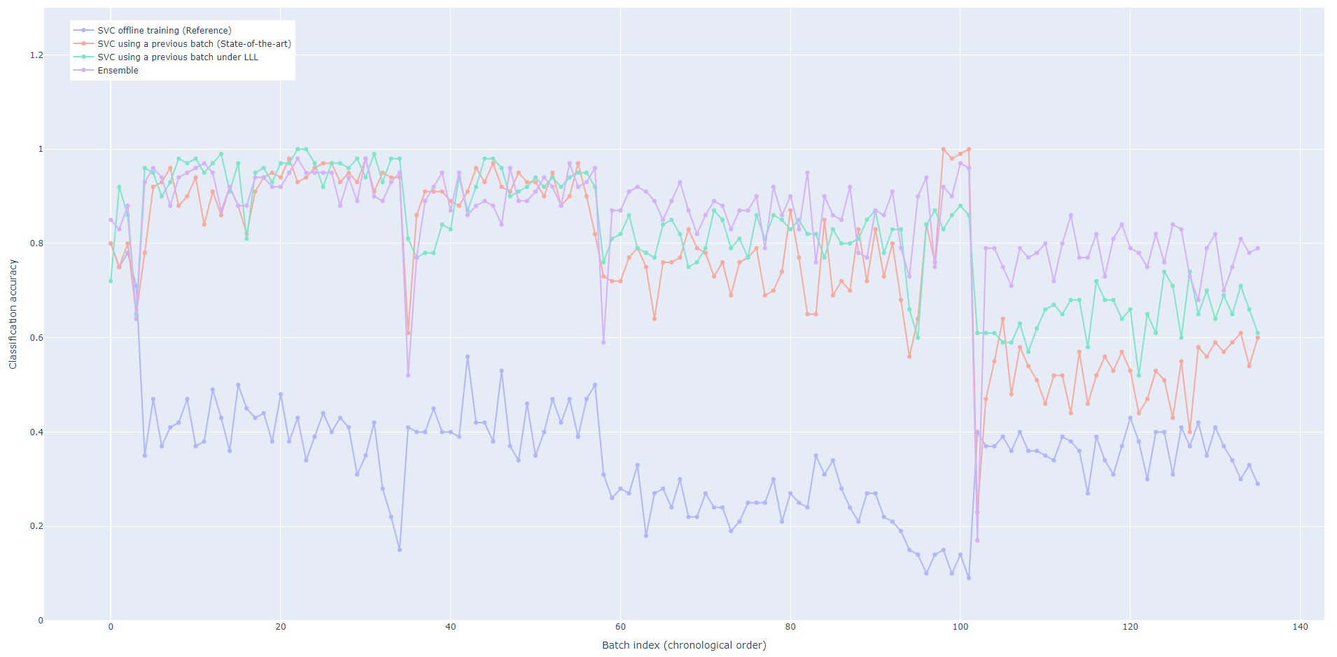
To illustrate the tool's capabilities with relevant data, we utilized the classification accuracy graph presented by Gheibi and Weyns[^1]. Although the graph is not included in their paper, it reflects the same reported results and can be accessed through the accompanying replication package[^2]. We added a fourth curve by incorporating the classification performance of an ensemble learner, complementing the three existing performance curves. Their study proposes a self-adaptive, lifelong machine learning model, demonstrating its effectiveness in classifying gas in a pipeline[^3][^4].
[^2]: Replication package for Gas Delivery Case Accessed: 2024-05-07
[^4]: Data: Gas Sensor Array Drift at Different Concentrations
Example 0 - The Input
To inspect the input that is provided to our tool, run
resmetric-cli ./example/fig.json
This is the input we are providing the tool:
Are these types of pictures not the thing you are looking for? Execution is not possible or taking too long?
In /example/plots/, you can find the interactive HTML files and print-ready versions of the plots .
Example 1 - Dip-Agnostic Resilience Metrics (AUC, Threshold)
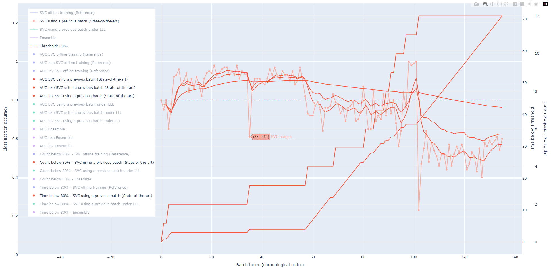
This example walks you through the most important dip-agnostic Resilience Metrics.
- Run
resmetric-cli --auc --count --time ./example/fig.json
- A browser tab will open and show the output. Use the legend to select the tracks you want to analyze. Double-click on the second entry "SVC using a previous batch (State-of-the-art)". This is the graph of normalized system performance. All other tracks will disappear.
- The Area Under Curve (AUC) is the weighted moving average of the normalized system performance. Select now the three traces "{AUC, AUC-exp, AUC-in} SVC using a previous batch (State-of-the-art)". They use three types of weighting 1) uniformly 2) with an exponential decay and 3) with an inverse distance weighting. With the latter two, more recent points contribute more to the average AUC at a given time.
- Now, select all traces in orange and the threshold line. This means, click on "Threshold: 80%", "Count below 80% - SVC using a previous batch (State-of-the-art)", and "Time below 80% - SVC using a previous batch (State-of-the-art)". A dashed line (the threshold) appears. The times are counted how often the normalized system performance dropped below the threshold (count) and how much time it spent there (time).
- To see all data, hover the x-axis (Batch Index (chronological order)) at around
x=0. By dragging towards the right side of your screen, you are able to scale the plot. - Try to use the button [≡] in the upper left corner. There you can toggle the legend.
Now, you see the image of above. You might also set the threshold by yourself with --treshold 70.
Metrics of this type are used when we do not care or cannot say when a dip starts (disruption) and ends (system adapted and recovered). A threshold is utilized if there is a defined or meaningful minimum tolerable performance.
If you want to explicitly save the plot as an HTML file, you can use --save followed by the desired path and filename.
For example:
resmetric-cli --auc --count --time --save example-1-plot.html ./example/fig.json
Example 2 - Robustness, Recovery Rate, and Recovery Ability
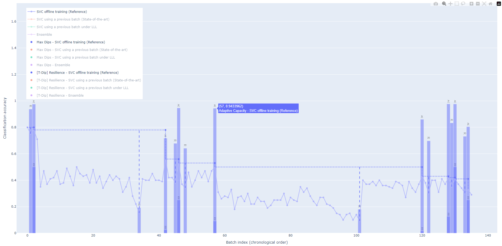
This example introduces Robustness (R), Recovery Rate (RR), and Adaptive Capacity (AC) as the first dip-dependent metrics. As a dip detection, we use maxima.
- Run
resmetric-cli --max-dips --bars ./example/fig.json
- Analogously as done in example 1, select the blue traces.
You can see annotated bars. They have the same acronyms as types above.
- Robustness (R) is meaningful if it is important that the system remains some minimal functionality
- The Recovery Rate (RR) might be employed when quick adaptation or short durations of performance gradation are required
- If the systems ability to recover after a disruption should be measured, the Adaptive Capacity (AC) will be the key metric.
Example 3 - Linear Regression with auto segmentation
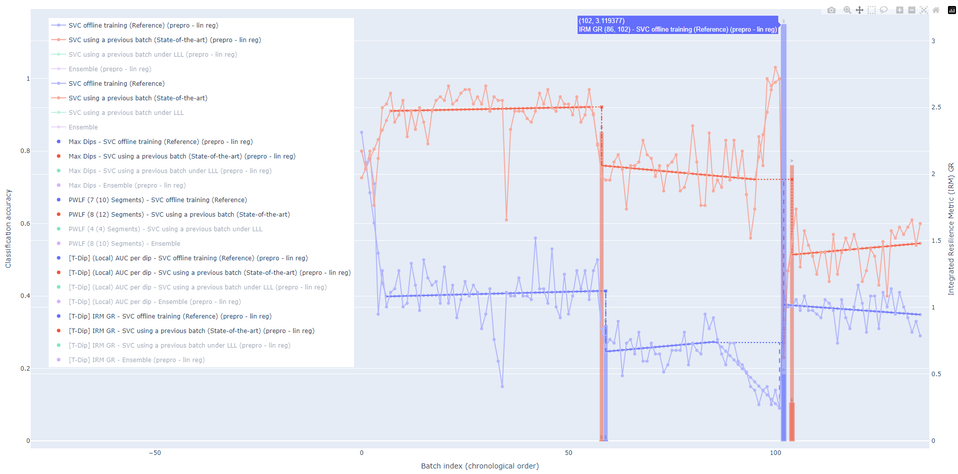
resmetric-cli --lin-reg --lin-reg-dips --dip-auc --irm ./example/fig.json
Before we start with the example, some foundations:
The biggest problem is that in a lot of setups, we do not have the exact times, when a disruption happened and therefore
where start and end the measurement is. If you have them though (through other priors or because you ran a controlled
environment--great! --manual-dips allows you to pass them!) For the not so lucky:
We assume that behind the noise, the system has steady phases. If the performance diminishes, there is a disruption.
This tool has multiple algorithms that try to detect these. The previous examples use the maxima-based
algorithm --max-dips. It is superfast and works without a prior. However, it is still susceptible to noise.
Another option is --threshold-dips. When the performance graph drops below a certain threshold, you have a dip.
It is also among the faster options. The by far slowest option delivers the best results, because it approximates
the function by linear regeression lines and keeps the ones with low slope:--lin-reg --lin-reg-dips. However, this
algorithm is the most robust against noise and the only algorithm that actuall
In this example, the AUC per dip and Integrated Resilience Metric (IRM) are calculated. The IRM is also called GR by Sansavini[^5]. (We adapted his formula by using TAPL+1 instead of TAPL.)
[^5]: G. Sansavini, "Engineering Resilience in Critical Infrastructures," in Resilience and Risk, I. Linkov and J. M. Palma-Oliveira, Eds., Dordrecht: Springer Netherlands, 2017, pp. 189–203, ISBN: 978-94-024-1123-2. DOI: 10. 1007/978-94-024-1123-2 6., Chapter 6, formula 6.12
Example 4 - Antifragility under u for dip-dependent metrics
Sometimes, we want to test if a Resilience Metric u improves over time. This is what we call the Degree of Antifragility under u: α_u (or alpha_u). It quantifies the monotonicity, i.e., the improvement of u. If α_u >=1, the system is antifragile and improves with each step. A higher number indicates faster improvement / growth of resilience. If 0 <= α_u <= 1, α_u indicates how monotonic increasing the system is. It is a membership function for antifragility. If α_u = 0, the resilience is strictly monotonically decreasing.
The analysis will depend on the Resilience Metric's sequence which depends on the start and end points of dips which in turn depends on the Dip Detection algorithm. So, be cautious with your assumptions. The following examples demonstrate the differences.
4a) Using Max Dips algorithm
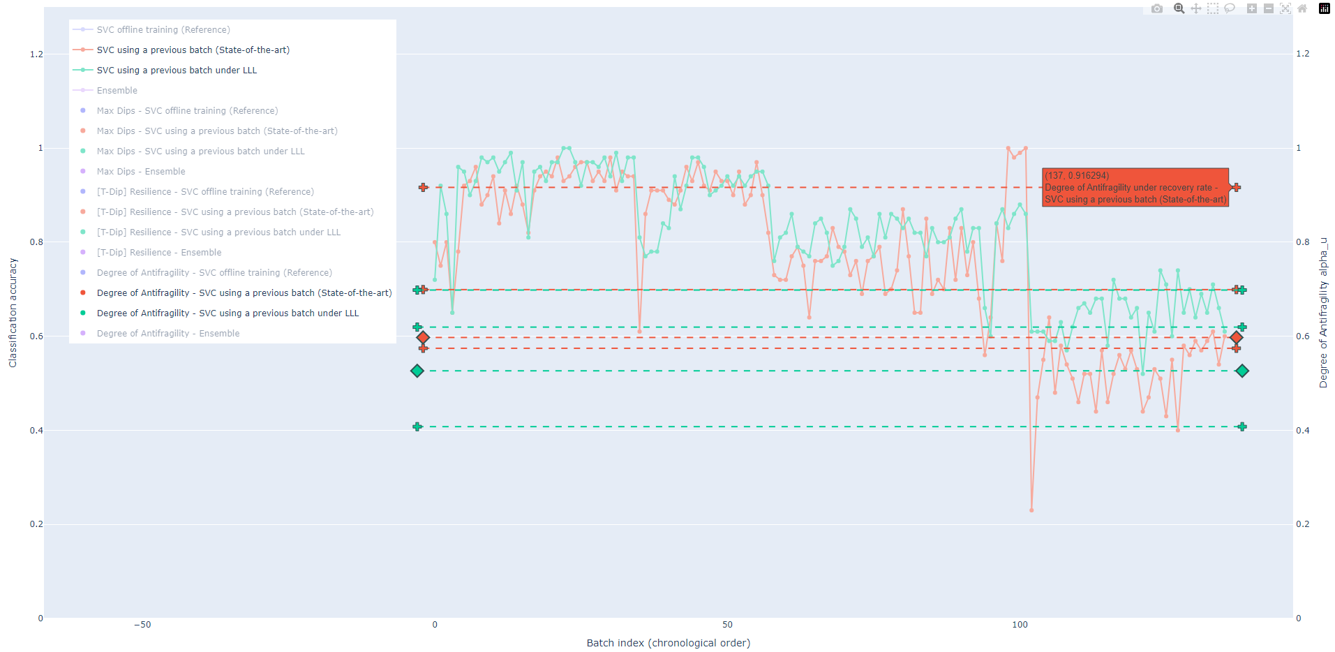
resmetric-cli --max-dips --bars --calc-res-over-time ./example/fig.json
Let's focus on the orange and green traces. As demonstrated in Example 2, --bars analyzes the robustness, recovery
rate and adaptive capacity. Therefore, the antifragility of those will be calculated.
Imagine that we take an overall resilience metric by taking the mean of each u. This allows us to calculate an overall degree of antifragility which is marked by the little diamond.
4b) Using linear regression dips
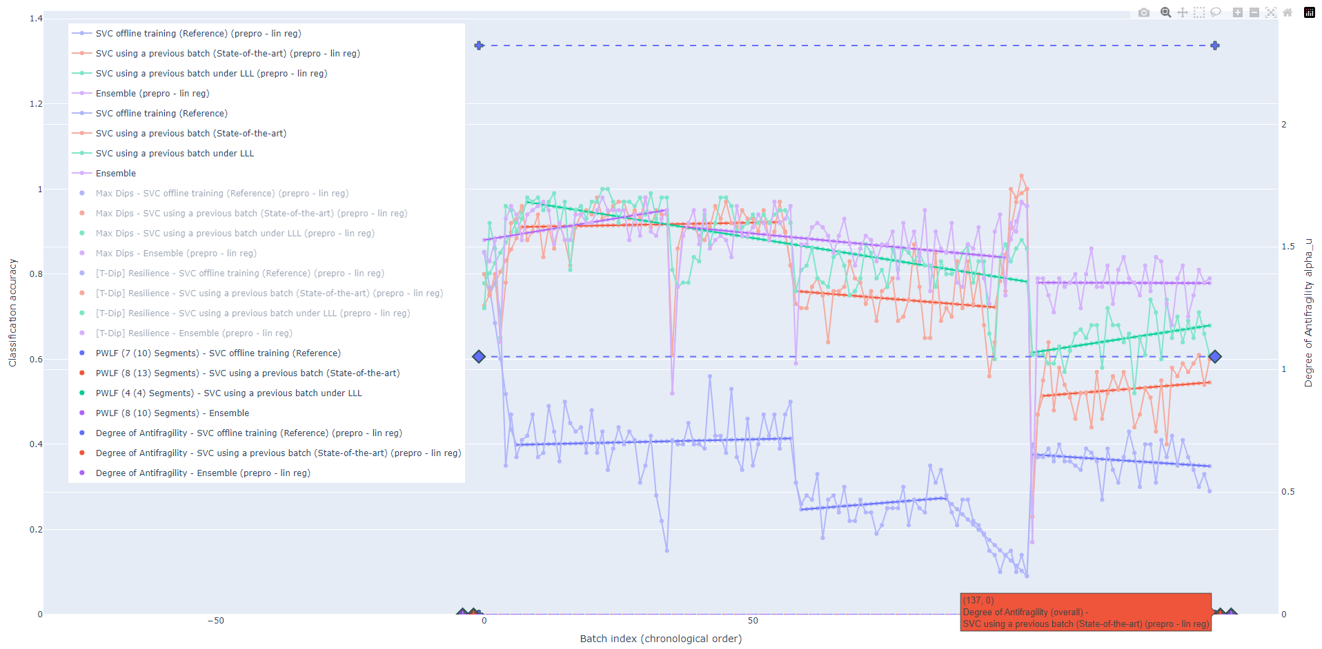
resmetric-cli --lin-reg --lin-reg-dips --bars --calc-res-over-time ./example/fig.json
In this result, the green trace just has one dip and therefore only one measure for a metric. Hence, α_u cannot be calculated and is also not displayed.
Comment on execution times
The calculations for the linear regression (--lin-reg --) take some minutes.
So take a small break or fill up your coffee cup meanwhile :)
In our example, the execution takes roughly 20 minutes for the four series of 136 data points each in the example file on a laptop with an Intel(R) Core(TM) i7-8650U CPU @ 1.90 GHz. Threshold Dips and Max Dips take $\sim 3s$ for the four series. (Both measured end to end, meaning from command to plot.) Conclusively, in our example, the linear regression dips algorithm is 400 times slower. Moreover, the calculation time grows faster (cubical, instead of linear and quadratic):
The linear regression uses Bayesian Optimization using Gaussian Processes and
takes $\mathcal{O}(tN^3 + tMN^2)$ (fitting + prediction), where $N$ are the samples (data points in a time series),
$M$ is the size of the search space (linear regression will have $m \in [1, M]$ segments;
the default for the upper bound $M$ is arbitrarily set to 20).
$t = 1.5 \cdot M \implies t \in \mathcal{O}(M)$ is the number of iterations (chosen arbitrarily).
Thus, $\mathcal{O}(MN^3 + M^2N^2)$.
As $M$ is user-set and small, it can be considered constant. This means the required time grows cubic to the
observations: $\mathcal{O}(N^3)$.
Threshold-based is in $\mathcal{O}(N)$. The Max Dips algorithm has a time complexity of $\mathcal{O}(N + k^2)$, where $k$ is the number of detected peaks within the series. Since data is noisy ( $k \in \mathcal{O}(N)$ ), one can assume $\mathcal{O}(N^2)$.
Assumptions
Right now, the code has the assumptions
- that the provided data is always 0 ≤ data ≤ 1 and
- that the time index starts with 0 and increments by 1 unit with each step
Demonstration cases
There are additional simple, synthetic cases to test the application in the folder /evaluation/.
Contributing and developing
Contributions are welcome! Please submit a pull request or open an issue on the GitHub repository.
Please check the development guide (README.md) and scripts in /development/
About
ResMetric is a Python module developed as part of my Master’s (M.Sc.) study project in Computer Science at Humboldt University of Berlin. It is a project within the Faculty of Mathematics and Natural Sciences, Department of Computer Science, Chair of Software Engineering.
This project was supervised by Marc Carwehl. I would like to extend my sincere gratitude to Calum Imrie from the University of York for his invaluable support and feedback.
The associated research paper is a collaborative effort.
— Ferdinand Koenig
License
ResMetric by Ferdinand Koenig is licensed under CC BY-NC-SA 4.0
This license requires that reusers give credit to the creator. It allows reusers to distribute, remix, adapt, and build upon the material in any medium or format, for noncommercial purposes only. If others modify or adapt the material, they must license the modified material under identical terms.
If you are interested in a commercial license, please contact me!
ferdinand (-at-) koenix.de
Appendix
Note: Installation on Ubuntu 23.04+, Debian 12+, and Similar OSs (error: externally-managed-environment)
Starting with Ubuntu 23.04, Debian 12, and similar systems, some operating systems have implemented
PEP 668 to help protect system-managed Python packages from being overwritten or
broken by pip-installed packages. This means that attempting to install Python packages globally
outside of a virtual environment can lead to errors such as error: externally-managed-environment.
This is not a bug with the resmetric package but rather expected behavior enforced by the operating system to keep
system packages stable. Generally, to install Python packages without issues, you must use a virtual environment.
If you encounter the installation error mentioning PEP 668 or error: externally-managed-environment, follow one of
the strategies below:
Option 1: Use the step-by-step installation guide
The virtual environment fixes this issue.
Option 2: Use pipx
- Install and setup
pipxsudo apt-get install -y pipx pipx ensurepath
- Install package via
pipxReplacepipbypipxin the installation command. This may look likepipx install resmetric
Make sure to use the right filename for the wheel file. - You are all set up!
Citation
Please cite both the associated paper and the ResMetric artifact when using the software.
@software{koenig_resmetric_artefact_2025,
  author        = {Koenig, Ferdinand},
  title         = {ResMetric: A Python Module for Visualizing Resilience and Antifragility},
  month         = jan,
  year          = 2025,
  publisher     = {Zenodo},
  doi           = {10.5281/zenodo.14724651},
  url           = {https://doi.org/10.5281/zenodo.14724651},
  license       = {CC BY-NC-SA 4.0}
}

@misc{koenig2025resmetricanalyzingresilienceenable,
  title         = {RESMETRIC: Analyzing Resilience to Enable Research on Antifragility},
  author        = {Ferdinand Koenig and Marc Carwehl and Calum Imrie},
  year          = {2025},
  eprint        = {2501.18245},
  archivePrefix = {arXiv},
  primaryClass  = {cs.SE},
  url           = {https://arxiv.org/abs/2501.18245}
}
Project details
Verified details
These details have been verified by PyPIProject links
GitHub Statistics
Maintainers
Release history Release notifications | RSS feed


Download files
Download the file for your platform. If you're not sure which to choose, learn more about installing packages.
Source Distribution
Built Distribution
Filter files by name, interpreter, ABI, and platform.
If you're not sure about the file name format, learn more about wheel file names.
Copy a direct link to the current filters
File details
Details for the file resmetric-1.0.0rc26.tar.gz.
File metadata
- Download URL: resmetric-1.0.0rc26.tar.gz
- Upload date:
- Size: 51.9 kB
- Tags: Source
- Uploaded using Trusted Publishing? Yes
- Uploaded via: twine/6.1.0 CPython/3.12.9
File hashes
| Algorithm | Hash digest | |
|---|---|---|
| SHA256 |
275cc411a2e25e469f635ad490c96e63ce9c10ba6236ebfabbddc2501ae5294e
|
|
| MD5 |
16309ec093a1341a47dfa290d8e3b5b7
|
|
| BLAKE2b-256 |
1aa1bd371b8d0f737ad9caff519240a2496d8ad485e51e677548cfc12adf61ba
|
Provenance
The following attestation bundles were made for resmetric-1.0.0rc26.tar.gz:
Publisher:
python-package-release.yml on ferdinand-koenig/resmetric
-
Statement:
-
Statement type:
https://in-toto.io/Statement/v1 -
Predicate type:
https://docs.pypi.org/attestations/publish/v1 -
Subject name:
resmetric-1.0.0rc26.tar.gz -
Subject digest:
275cc411a2e25e469f635ad490c96e63ce9c10ba6236ebfabbddc2501ae5294e - Sigstore transparency entry: 199340686
- Sigstore integration time:
-
Permalink:
ferdinand-koenig/resmetric@63659da1e9cdd7b5cacaec57e227df5f0e8d9551 -
Branch / Tag:
refs/heads/release - Owner: https://github.com/ferdinand-koenig
-
Access:
public
-
Token Issuer:
https://token.actions.githubusercontent.com -
Runner Environment:
github-hosted -
Publication workflow:
python-package-release.yml@63659da1e9cdd7b5cacaec57e227df5f0e8d9551 -
Trigger Event:
push
-
Statement type:
File details
Details for the file resmetric-1.0.0rc26-py3-none-any.whl.
File metadata
- Download URL: resmetric-1.0.0rc26-py3-none-any.whl
- Upload date:
- Size: 43.2 kB
- Tags: Python 3
- Uploaded using Trusted Publishing? Yes
- Uploaded via: twine/6.1.0 CPython/3.12.9
File hashes
| Algorithm | Hash digest | |
|---|---|---|
| SHA256 |
3fb9d76f6e85d2087c516a312aa523d379fff6a4a097c9793f71d6cb4fdcf54c
|
|
| MD5 |
dc44584fbd2a0a7f272e188b12110f2c
|
|
| BLAKE2b-256 |
b1195115cb2d1aa7d2e0cb8c36a6d066b7e4aed2aa406fd3b2b3c50f57722fb3
|
Provenance
The following attestation bundles were made for resmetric-1.0.0rc26-py3-none-any.whl:
Publisher:
python-package-release.yml on ferdinand-koenig/resmetric
-
Statement:
-
Statement type:
https://in-toto.io/Statement/v1 -
Predicate type:
https://docs.pypi.org/attestations/publish/v1 -
Subject name:
resmetric-1.0.0rc26-py3-none-any.whl -
Subject digest:
3fb9d76f6e85d2087c516a312aa523d379fff6a4a097c9793f71d6cb4fdcf54c - Sigstore transparency entry: 199340695
- Sigstore integration time:
-
Permalink:
ferdinand-koenig/resmetric@63659da1e9cdd7b5cacaec57e227df5f0e8d9551 -
Branch / Tag:
refs/heads/release - Owner: https://github.com/ferdinand-koenig
-
Access:
public
-
Token Issuer:
https://token.actions.githubusercontent.com -
Runner Environment:
github-hosted -
Publication workflow:
python-package-release.yml@63659da1e9cdd7b5cacaec57e227df5f0e8d9551 -
Trigger Event:
push
-
Statement type:


