Rule-based 3D geological reservoir modeling

Project description
ResMill
Rule-based 3D geological reservoir modeling in Python.


Created by Ilgar Baghishov and Elnara Rustamzade.
ResMill generates geologically plausible synthetic 3D reservoir models — turbidite lobes, fluvial channel systems, deltas, and Gaussian heterogeneity fields — from a handful of physical parameters, with no commercial software required. It is a Python-native, pip-installable tool for subsurface modeling in oil & gas, groundwater, and carbon-storage workflows.
The modeling engines are derived from two established bodies of work:
- Fluvial / channel / delta engine — ported from ALLUVSIM, the event-based fluvial simulator of Michael J. Pyrcz, Jeff B. Boisvert, and Clayton V. Deutsch (Pyrcz et al., 2009).
- Turbidite-lobe generation — based on the rule-based lobe models of Wen Pan, Honggeun Jo, and Michael J. Pyrcz (Jo & Pyrcz, 2019; Jo et al., 2021).
See References for full citations.
Install
pip install resmill
For development (tests, notebooks):
git clone https://github.com/IlgarBaghishov/ResMill.git
cd ResMill
pip install -e ".[dev]"
Requires Python ≥ 3.10. Dependencies: NumPy, SciPy, Numba, Matplotlib.
Quick start
import resmill as rm

# A layer owns only its grid geometry (sizes in metres).
lobe = rm.LobeLayer(nx=64, ny=64, nz=32, x_len=640, y_len=640, z_len=32, top_depth=5000)

# create_geology() runs the physics and fills the property arrays.
lobe.create_geology(poro_ave=0.20, perm_ave=1.5, poro_std=0.03, perm_std=0.5, ntg=0.7)

# Outputs are (nx, ny, nz) numpy arrays:
lobe.poro_mat   # porosity, 0–1
lobe.perm_mat   # permeability, mD
lobe.active     # 0/1 reservoir (sand) mask
lobe.facies     # facies-class codes

# Built-in visualization (3 orthogonal slices as a cube):
rm.plot_cube_slices(lobe, title="Turbidite lobes")
How it works
ResMill has three core pieces:
-
Layer— the base class. A layer is constructed with grid geometry only:nx, ny, nz(cell counts),x_len, y_len, z_len(extent in metres),top_depth(metres), and optionaldip. No physics in the constructor. -
create_geology(...)— each layer type implements this. It runs the rule-based / stochastic engine and populates the property arrays. All physics parameters live here, not in__init__. -
Reservoir([layer_top, …, layer_bottom])— stacks layers vertically into one model. Layers are listed top → bottom; every layer must share the samenx, ny, x_len, y_len, and each layer's base depth must equal the next layer'stop_depth(the constructor validates this).
All arrays are shaped (nx, ny, nz) using meshgrid(..., indexing='ij').
Output properties
| Attribute | Meaning | Units / values |
|---|---|---|
poro_mat |
porosity | linear 0–1 |
perm_mat |
permeability | mD (linear) |
active |
reservoir (sand) mask | 0 / 1 |
facies |
facies class | see table below |
facies semantics vary by layer: channel/delta use the full multi-class Alluvsim
codes; LobeLayer.facies is a lobe index; GaussianLayer has no multi-class facies
— use active for its sand mask.
⚠️ Permeability units gotcha. For
LobeLayerandGaussianLayer, theperm_ave/perm_stdinputs are in log10(mD) space (e.g.perm_ave=1.5→ ~32 mD mean; sensible range0–4). The outputperm_matis still linear mD. Passing a linear value likeperm_ave=500overflows and saturates the output.poro_ave/poro_stdstay in linear0–1.
Interpreting the figures
Every gallery image below is a 1×3 panel through the mid-planes of the model:
- XY — map view (plan view) at mid-depth.
- XZ and YZ — vertical cross-sections.
Sections follow the library's own convention (rm.plot_slices, rm.plot_cube_slices,
origin='lower'): the vertical axis is the Z cell index increasing upward, so the
top of the deposited interval is at the top of each section and the base is at the
bottom.
Channel and delta models are coloured by the Alluvsim facies classes:
| Code | Facies | Description |
|---|---|---|
-1 |
FF | floodplain (non-reservoir background) |
0 |
FFCH | abandoned-channel mud plug |
1 |
CS | crevasse splay |
2 |
LV | levee |
3 |
LA | lateral-accretion point bar |
4 |
CH | active channel fill |
The facies are ordered by reservoir quality (FF < FFCH < CS < LV < LA < CH).
All gallery figures are reproducible from a clean checkout with
docs/make_readme_figures.py.
Shared setup for the gallery snippets
Every snippet below assumes this preamble:
import resmill as rm

# Standard 64×64×32 grid (640×640×32 m).
GRID = dict(nx=64, ny=64, nz=32, x_len=640, y_len=640, z_len=32, top_depth=0)
Gallery — geology types and presets
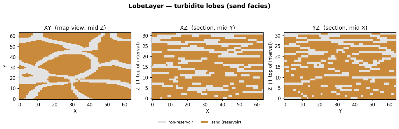
LobeLayer — turbidite lobes
Deep-water lobes deposited by sediment-gravity flows, with compensational stacking (younger lobes preferentially fill topographic lows), optional upthinning toward lobe margins, and Bouma-sequence grading. Produces clean sand lobe bodies in a mud background.
lobe = rm.LobeLayer(**GRID)
lobe.create_geology(poro_ave=0.20, perm_ave=1.5, poro_std=0.03, perm_std=0.5,
                    ntg=0.7, r_ave=180, r_std=30, asp=1.5, upthinning=True)
rm.plot_slices(lobe)
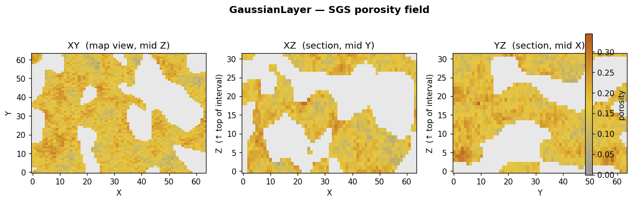
GaussianLayer — SGS heterogeneity field
Sequential Gaussian simulation produces a spatially-correlated continuous porosity/permeability field, thresholded to a target net-to-gross. Use it as a heterogeneous background or for sand/shale distributions without discrete geobodies.
gauss = rm.GaussianLayer(**GRID)
gauss.create_geology(poro_ave=0.18, perm_ave=1.5, poro_std=0.04, perm_std=0.5, ntg=0.6)
rm.plot_slices(gauss.poro_mat, axis=2)   # Z slices of the porosity field
ChannelLayer — fluvial systems
A single, faithful port of the ALLUVSIM event-based engine: channels meander,
migrate, avulse, cut off oxbows, and build levees and crevasse splays. Behaviour is
driven by importable presets that reproduce Pyrcz's canonical fluvial reservoir
architectures — pass any preset with **PRESET and override individual parameters as
needed.
from resmill.layers.channel import (
    PV_SHOESTRING, CB_JIGSAW, CB_LABYRINTH, SH_DISTAL, SH_PROXIMAL, MEANDER_OXBOW,
)
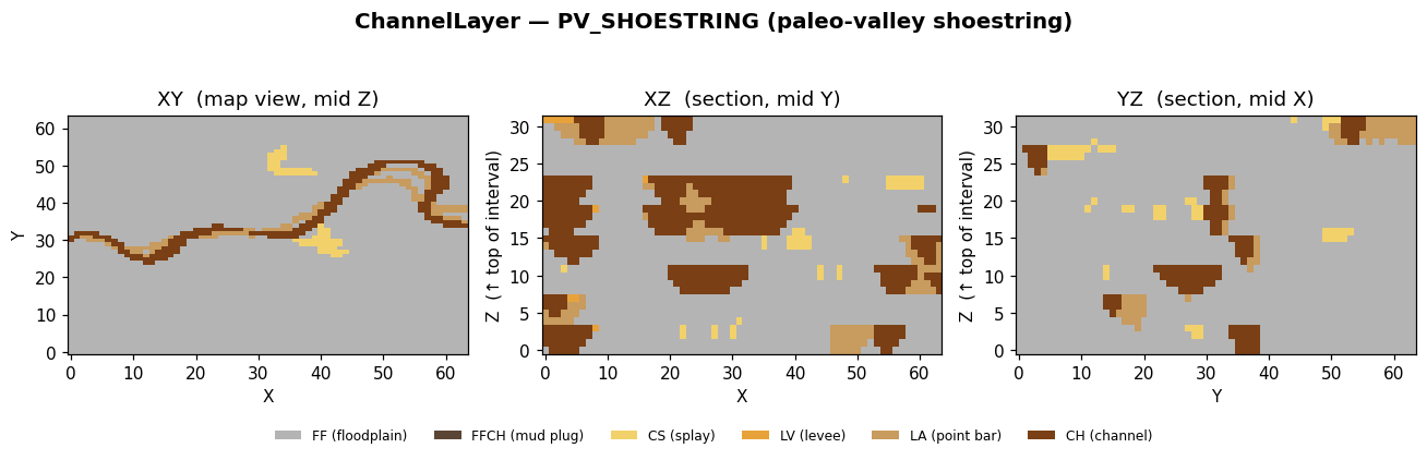
PV_SHOESTRING — paleo-valley shoestring
Low net-to-gross (~0.10): a single high-sinuosity channel with prominent lateral-accretion point bars, leaving isolated "shoestring" sand bodies encased in floodplain mud.
ch = rm.ChannelLayer(**GRID)
ch.create_geology(seed=42, **PV_SHOESTRING)
rm.plot_slices(ch)
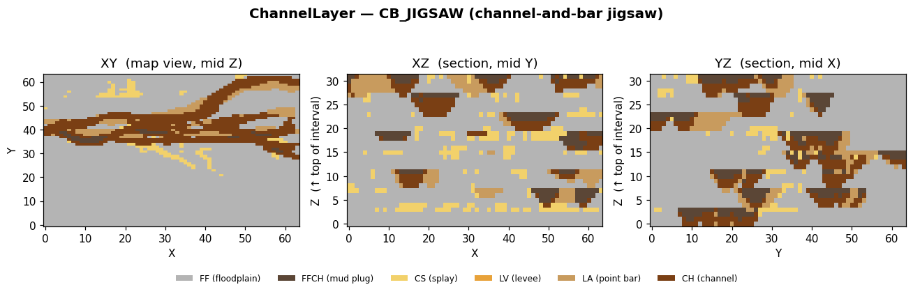
CB_JIGSAW — channel-and-bar jigsaw
Moderate NTG (~0.30) with heavy avulsion-inside, so channel-and-bar bodies amalgamate and interlock like a jigsaw, separated by FFCH mud plugs.
ch = rm.ChannelLayer(**GRID)
ch.create_geology(seed=42, **CB_JIGSAW)
rm.plot_slices(ch)
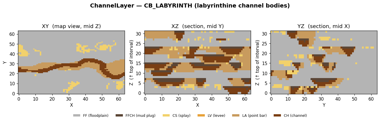
CB_LABYRINTH — labyrinthine channel bodies
Many aggradation events with low avulsion, giving isolated, poorly-connected channel bodies threaded through mud — a labyrinthine connectivity pattern.
ch = rm.ChannelLayer(**GRID)
ch.create_geology(seed=42, **CB_LABYRINTH)
rm.plot_slices(ch)
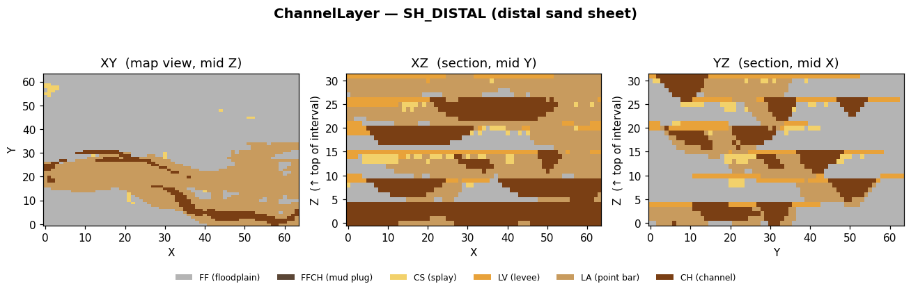
SH_DISTAL — distal sand sheet
High NTG (~0.50) with thick levee blankets, producing sheet-like, well-connected distal sandstone.
ch = rm.ChannelLayer(**GRID)
ch.create_geology(seed=42, **SH_DISTAL)
rm.plot_slices(ch)
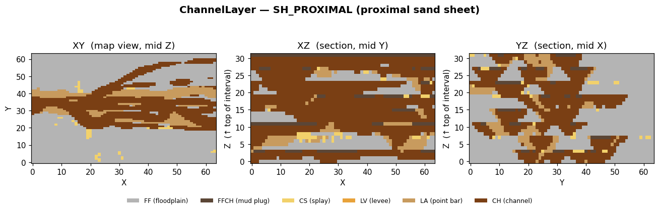
SH_PROXIMAL — proximal sand sheet
High NTG (~0.40) from heavy avulsion plus wide, shallow channels that amalgamate into a proximal sand sheet.
ch = rm.ChannelLayer(**GRID)
ch.create_geology(seed=42, **SH_PROXIMAL)
rm.plot_slices(ch)
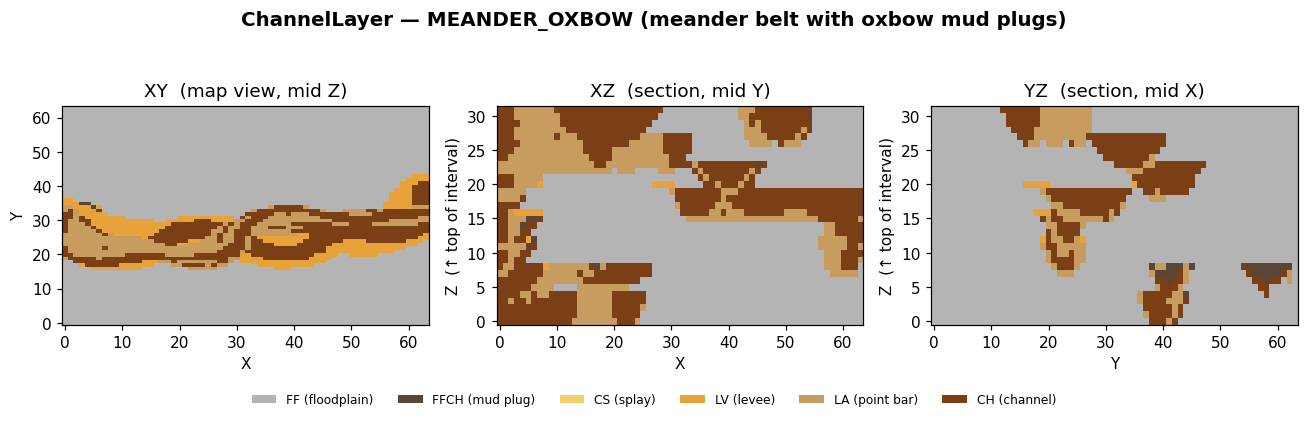
MEANDER_OXBOW — meander belt with oxbow mud plugs
A single sinuous channel that migrates across the floodplain until tight bends neck-cut into oxbow loops; each cutoff is painted as an FFCH mud plug, giving the classic neck-cutoff → oxbow lake → mud-plug succession stacked into a multi-storey meander belt.
ch = rm.ChannelLayer(**GRID)
ch.create_geology(seed=42, **MEANDER_OXBOW)
rm.plot_slices(ch)
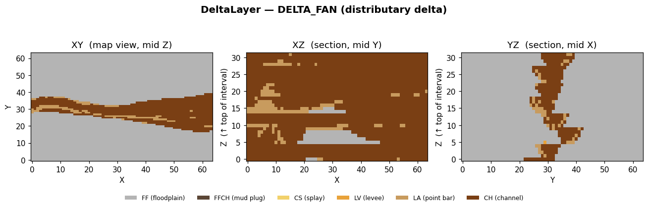
DeltaLayer — distributary delta
Built on the same fluvial engine (defaults from the DELTA_FAN preset): a trunk
channel that bifurcates into a distributary network fanning across the grid, stacked
over several generations. Knobs like trunk_length_fraction, progradation_fraction,
branch_spread_deg, and paint_mouth_bars shape the fan.
delta = rm.DeltaLayer(**GRID)
delta.create_geology(seed=3)            # DELTA_FAN defaults are applied automatically
rm.plot_slices(delta)
Stacking layers into a reservoir
Layers are stacked top → bottom; each layer's base depth must meet the next
layer's top_depth.
import resmill as rm
from resmill.layers.channel import MEANDER_OXBOW

nx, ny, x_len, y_len = 64, 64, 640, 640

# Top: delta fan, 10 m thick (5000–5010 m)
top = rm.DeltaLayer(nx=nx, ny=ny, nz=10, x_len=x_len, y_len=y_len, z_len=10, top_depth=5000)
top.create_geology(seed=3)

# Middle: turbidite-lobe blanket, 10 m thick (5010–5020 m)
mid = rm.LobeLayer(nx=nx, ny=ny, nz=10, x_len=x_len, y_len=y_len, z_len=10, top_depth=5010)
mid.create_geology(poro_ave=0.20, perm_ave=1.5, poro_std=0.03, perm_std=0.5, ntg=0.7)

# Bottom: meander belt with oxbow mud plugs, 12 m thick (5020–5032 m)
bot = rm.ChannelLayer(nx=nx, ny=ny, nz=12, x_len=x_len, y_len=y_len, z_len=12, top_depth=5020)
bot.create_geology(seed=1, **MEANDER_OXBOW)

reservoir = rm.Reservoir([top, mid, bot])
print(reservoir.poro_mat.shape)         # (64, 64, 32)
rm.plot_cube_slices(reservoir.poro_mat, title="Stacked reservoir — porosity")
Layer & preset reference
| Layer | Preset(s) | Geology |
|---|---|---|
LobeLayer |
— | Turbidite lobes; compensational stacking, upthinning, Bouma grading |
GaussianLayer |
— | SGS continuous porosity/perm heterogeneity field |
ChannelLayer |
PV_SHOESTRING |
Isolated shoestring channel sands (low NTG) |
CB_JIGSAW |
Amalgamated channel-and-bar jigsaw | |
CB_LABYRINTH |
Isolated labyrinthine channel bodies | |
SH_DISTAL |
Distal sheet sandstone (high NTG) | |
SH_PROXIMAL |
Proximal amalgamated sand sheet | |
MEANDER_OXBOW |
Multi-storey meander belt with oxbow mud plugs | |
DeltaLayer |
DELTA_FAN |
Prograding distributary-fan delta |
Channel presets are plain dicts — start from one and override any parameter, e.g.
ch.create_geology(seed=0, **PV_SHOESTRING, NTGtarget=0.15).
References
If you use ResMill in published work, please cite the methods it is built on:
- ALLUVSIM (fluvial / channel / delta engine): Pyrcz, M. J., Boisvert, J. B., & Deutsch, C. V. (2009). ALLUVSIM: A program for event-based stochastic modeling of fluvial depositional systems. Computers & Geosciences, 35(8), 1671–1685.
- Rule-based lobe models: Jo, H., & Pyrcz, M. J. (2019). Robust Rule-Based Aggradational Lobe Reservoir Models. Natural Resources Research, 29(2), 1193–1213.
- Deep-water lobe modeling: Jo, H., Pan, W., Santos, J. E., Jung, H., & Pyrcz, M. J. (2021). Machine Learning Assisted History Matching for a Deepwater Lobe System. Journal of Petroleum Science and Engineering, 207, 109086.
License
MIT — see LICENSE.


Download files
Download the file for your platform. If you're not sure which to choose, learn more about installing packages.
Source Distribution
Built Distribution
Filter files by name, interpreter, ABI, and platform.
If you're not sure about the file name format, learn more about wheel file names.
Copy a direct link to the current filters
File details
Details for the file resmill-0.1.2.tar.gz.
File metadata
- Download URL: resmill-0.1.2.tar.gz
- Upload date:
- Size: 89.4 kB
- Tags: Source
- Uploaded using Trusted Publishing? No
- Uploaded via: twine/6.2.0 CPython/3.12.9
File hashes
| Algorithm | Hash digest | |
|---|---|---|
| SHA256 |
eb49919f1e097c1c231db75ad47bf7c6cc010d599940841747a31c768286d1cb
|
|
| MD5 |
5466f6a703758cd45d5a2a9b60d65dc7
|
|
| BLAKE2b-256 |
54631583f556084ae96ba94c406b1f4144d52c41a0be51572526c6db6c856ed7
|
File details
Details for the file resmill-0.1.2-py3-none-any.whl.
File metadata
- Download URL: resmill-0.1.2-py3-none-any.whl
- Upload date:
- Size: 84.7 kB
- Tags: Python 3
- Uploaded using Trusted Publishing? No
- Uploaded via: twine/6.2.0 CPython/3.12.9
File hashes
| Algorithm | Hash digest | |
|---|---|---|
| SHA256 |
6a79cd7f6f323336c92f2ebdd6142d722aae050eff88ace8dd8df33d4b55e74c
|
|
| MD5 |
e6f3de6debec2a90cad142bbd5652193
|
|
| BLAKE2b-256 |
8f49f24704e6a2ed12665a67285543c53e3b5a7d46aa2422bb2469987221844e
|


