The FFT of operators: probe, compose, read — matrix-free spectral computation with a built-in cost law.

Project description
resona — the FFT of operators
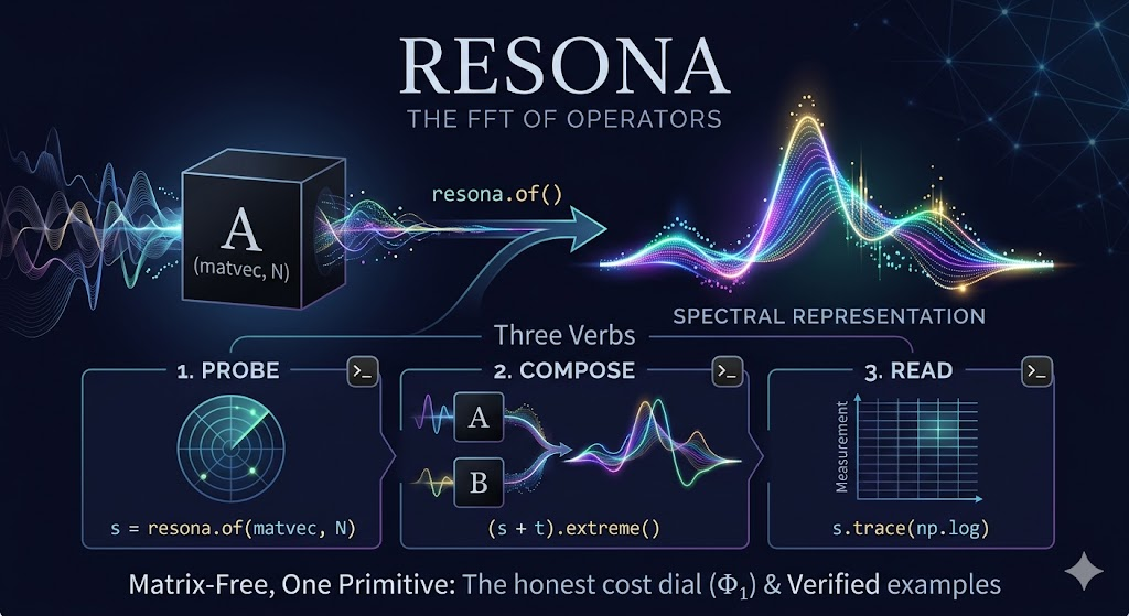
fft(x)takes a signal to the basis where convolution becomes pointwise multiply.resona.of(A)takes an operator (anything that can multiply a vector) to the representation where composition becomes addition — and from which every spectral question is answered. No matrix is ever formed;eigis never called.
In plain words: you have a thing that transforms vectors — a matrix too
big to write down, a graph, a physics simulation, a neural network's Hessian, a
quantum Hamiltonian. resona listens to it, tells you everything about its
spectrum, lets you add and multiply such things without ever building them,
apply functions of them to vectors, measure how hard your problem truly is —
and even design new operators to order.
pip install resona # numpy + scipy only
60 seconds
import numpy as np, resona

A = np.random.default_rng(0).standard_normal((3000, 3000)); A = A @ A.T / 3000
matvec = lambda v: A @ v        # ← all resona ever needs: v ↦ Av

s = resona.of(matvec, 3000)     # PROBE  — "ring" the operator, hear its spectrum
s.extreme()                     # smallest & largest eigenvalue
s.trace(np.log)                 # log-determinant — no Cholesky, no eig
s.density(np.linspace(0, 4, 200))   # the spectrum's shape
s.effective_rank()              # the cost dial: is this problem cheap or hard?

t = resona.of(lambda v: A @ (A @ v), 3000)
(s + t).extreme()               # spectrum of A + A², A + A² never formed

b = np.random.standard_normal(3000)
mv1 = lambda v: A @ v + v                        # A + I (well-conditioned)
x = resona.apply(mv1, lambda lam: 1/lam, b)      # solve (A+I)x = b, matrix-free
Every line above is matrix-free: the cost is the matvec, not O(N³).
Choose your door
🚶 New to operators / numerics? Take the tour — ten stops from "what is a matvec" to designing your own operators, every stop in plain words first, the math second.

🎓 Mathematician? The library is a dictionary of theorems made executable —
each entry verified in tests/ and examples/ against dense ground truth:
| you call | which is | verified |
|---|---|---|
resona.of(mv, N) |
stochastic Lanczos quadrature = Gauss quadrature of the spectral measure | moments vs dense, 35-operator suite |
s + t, s @ t |
exact closure (A+B)x = Ax+Bx; at the measure level: free convolution ⊞/⊠ (Voiculescu) |
extreme eig of A+B to 1e-9 |
s.boxplus(t) |
κₙ(A⊞B) = κₙ(A)+κₙ(B) (Speicher, non-crossing partitions); as_spectral=True → Golub–Welsch |
semicircle ⊞ semicircle exact |
s.r(w) / s.s(w) |
R-transform (linearizes ⊞ — "its Cole–Hopf", our framing, see NOVELTY) / S-transform (⊠) | additivity to 0.5% |
s.flow(t, xs) |
free heat flow = inviscid complex Burgers; shock_time = band merger |
t_c ≈ 1 for atoms ±1 |
subordination.pastur_grid |
the Pastur subordination fixed point g = G_A(z−σ²g) |
m₂ vs Monte-Carlo |
s.extreme() |
BBP transition & Tracy–Widom fluctuations live here | λ=θ+1/θ above θ_c; measured exp −0.65 (theory −⅔) |
defect.pseudospectrum_radius |
the ε^{1/q} bloom of an order-q Jordan defect; GMRES follows Λ_ε | exact on J_q, q=2…5 |
solve.catastrophe_solve |
Arnold A_{q−1} stratum ⇒ float64 keeps 16/q digits; budget dps = q·target | 4.9 → 17.0 digits |
cost.level_spacing_ratio |
⟨r⟩: Poisson 0.386 (integrable) vs GOE 0.531 (chaotic) | 0.392 / 0.532 on XXZ±NNN |
lift.conserved_charge |
commutator-Gram eigenproblem: near-kernel = integrals of motion | finds H, ΣZ, bilinears blind |
lift.carleman_* |
Carleman linearization; over GF(p), x^p≡x makes ANY logic exactly linear | 0 errors on all pⁿ inputs |
from_measure / from_eigenbasis |
the inverse spectral problem (Stieltjes / Jacobi); synthesis of operators to order | eig = order to 5.6e-15 |
s.effective_rank() |
Φ₁ participation ratio; the Extraction-Law cost dial | dequantization boundary (Tang) |
free.rie_clean |
free DEconvolution: Ledoit–Péché / Bun–Bouchaud–Potters RIE | 95% of the oracle at q=1/2 |
s.trace(f, with_err=True) |
the stochastic estimate with its own standard error (probe scatter) | bars bracket truth, free |
quadform(..., certified=True) |
Gauss–Radau brackets (Golub–Meurant): the answer PROVABLY inside | GP variance certified, width 4e-4 at k=24 |
s.zoom(a, b) |
Chebyshev spectrum slicing: interior eigenvalues at full k-resolution | interior to 4e-16 of span |
of(deflate=K) |
Hutch++ at the measure level: exact top-K atoms + complement probes | variance −63× (Tr A²), −724× (Tr eᴬ) |
of(engine="kpm") |
Chebyshev/Jackson harvest, no reorthogonalization | 2.7× at k=256, same object out |
cloud(mv, N) |
non-Hermitian Arnoldi cloud; abscissa = NUMERICAL abscissa (transient growth) | Markov gap to 1e-3; ω−α gap measured |
lift.koopman(X) |
data → the DMD/Koopman propagator's action (one thin SVD) | rotation eigenvalues to 1e-6 |
thermal.correlator |
typicality: ⟨O(t)O⟩_β with two Krylov evolutions per point | vs dense to 0.014 (200 probes) |
🔧 Have a task right now? The cookbook: find your task in the "I want to…" table, copy the recipe.
What it solves (matrix-free, one primitive)
Verified against dense ground truth in examples/ — 44 gallery
scripts, every metric printed by the script itself:
| task | what | metric |
|---|---|---|
| GP log-determinant | log|K| for hyperparameter learning at scale |
0.84% rel.err, no Cholesky |
| Loss-Hessian spectrum | sharpness & curvature from HVPs, no Hessian formed | λ_max 0.00%, Tr 0.30% |
| Spectrum of A+B | composed, matrix-free (Horn's problem in practice) | extreme eig to 1e-9 |
| Deep-net trainability | cond(W_L…W_1) predicted from init, no fwd/bwd |
Gaussian explodes, orthogonal ≈1 |
| Effective rank Φ₁ | the cost dial: structured/cheap vs full/frontier | 14 vs 466 |
| Nonlinear PDE (Burgers) | lift to linear (Cole–Hopf) → exp(tK)·v |
residual 5e-9, matrix-free |
| 35 operators → spectra | matrix-free Ritz seed → Rayleigh polish | seed 1e-4 → 1e-16, 100% machine-zero |
| Operator synthesis | order a spectrum → get a working local matvec | eig = order to 5.6e-15 |
| GMRES stall prediction | same spectrum, opposite fates — the pseudospectrum knows | 14 iters vs stall, read from σ_min |
| Is it integrable? | ⟨r⟩ + blind conserved-charge search | 0.392/0.532; 4 charges vs 1 |
| Signal in noise (BBP) | does a spike detach from the bulk? | λ=θ+1/θ above θ_c=1 |
| Anderson localization | metal→insulator from disorder, matrix-free | Λ: 0.97→0.15 in 3.4s |
| Tracy–Widom edge | the universal fluctuation law of extreme() |
std·N^⅔→1.27, measured exp −0.65 (theory −⅔) |
| JWST image analysis | structure map, source detection, denoising — straight from PyPI | corr 0.97 vs dense; front found |
| Covariance cleaning (RIE) | free deconvolution of Marchenko–Pastur noise | 1.81× closer to truth, 95% of oracle |
| The zeta-zero operator | Hilbert–Pólya computationally: built, verified, interrogated | eig = zeros to 2.8e-13; β-rigidity > GUE |
More broadly: density of states, Tr f(A) (log-det, Tr A⁻¹, partition
functions, Schatten norms), extreme eigenvalues & gaps, disorder-averaged
spectra, phase transitions, spectral clustering, operator design — anything that
is a spectral functional of an operator you can only matvec.
The shape of the library
Three verbs on one object, everything else reads off the same hub:
  PROBE                       READ                          COMPOSE
  s = resona.of(matvec, N) →  s.trace(f) s.density(xs)      s + t   s @ t
                              s.extreme() s.moment(p)       s.boxplus(t)
                                   │
  the lifted coordinates:          │        the dials:
  s.cauchy(z) s.r(w) s.s(w)        │        s.effective_rank()  (Φ₁)
  s.cumulants()                    │        s.condition()
                                   │
  the flow:  s.flow(t, xs)  s.shock_time()      the closure:  s.levels(N)

  APPLY      resona.apply(matvec, f, v)  →  f(A)·v   (solve / evolve / filter)
  INVERSE    resona.from_measure / from_eigenbasis   (measure → operator: SYNTHESIS)
  PRECISION  resona.solve.rayleigh_polish / catastrophe_solve  (digits, only where needed)
When the matvec also maps blocks (A @ X), probing rides one BLAS-3
block-Lanczos automatically — 2–4× faster, bit-compatible (verified, then
enabled; never assumed).
The deeper machinery is in plain modules — wkernel (spectral Jacobian
∂λ/∂k + design), lift (R/S transforms, Carleman, conserved charges), free
(cumulants, freeness), subordination (Pastur), flow (Burgers), beta
(max-entropy closure), defect (Richardson + pseudospectra), cost
(Extraction Law, ⟨r⟩), solve (precision on the defect) — each documented in
its docstring, each verified in tests/.
Honesty
The underlying algorithms (SLQ, Lanczos, free probability, Carleman,
Golub–Welsch) are classical and credited in NOVELTY.md.
resona's contribution is the single primitive + matrix-free composition
algebra + the built-in cost law as one object — the way FFT organizes signal
processing. The unifying claims (the Extraction Law, Φ₁-as-boundary) are
research hypotheses, labelled as such; the computations are verified. Every
estimate states its honest limit in its docstring: condition() is a lower
bound, boxplus needs freeness, from_measure is ill-conditioned for atomic
measures, catastrophe_solve cannot recover information float64 already
destroyed. Stochastic reads give ~2–4 digits; machine precision is bought,
where it matters, with rayleigh_polish — paying only on the defect's support.
Theory
The unified picture — the response measure as a conjugate pair, free
probability (closure, the freeness boundary, the semicircle attractor), the
defect = shock = edge identity, and the Extraction Law — is in
THEORY.md, with reproducible scripts in theory/.
The claims are calibrated in NOVELTY.md; open conjectures and
the research log including the failures are in FRONTIER.md.
The cost of every method is in COMPLEXITY.md.
License
MIT © 2026 Dmitry Sierikov. Attribution requested for the research
contributions in NOVELTY.md.
Release history Release notifications | RSS feed


Download files
Download the file for your platform. If you're not sure which to choose, learn more about installing packages.
Source Distribution
Built Distribution
Filter files by name, interpreter, ABI, and platform.
If you're not sure about the file name format, learn more about wheel file names.
Copy a direct link to the current filters
File details
Details for the file resona-1.2.0.tar.gz.
File metadata
- Download URL: resona-1.2.0.tar.gz
- Upload date:
- Size: 66.3 kB
- Tags: Source
- Uploaded using Trusted Publishing? No
- Uploaded via: twine/6.2.0 CPython/3.10.12
File hashes
| Algorithm | Hash digest | |
|---|---|---|
| SHA256 |
f7073a4299d56daf6e1e2735c461e7eda056a52e3b04a0ac49f68525d196ed93
|
|
| MD5 |
06844937de6fc0e7f55c094d9f51f9a8
|
|
| BLAKE2b-256 |
d1cc5506057f77ff7c3da4c465f8f01b11990d29ea7c80e9f9eb39072fcd4521
|
File details
Details for the file resona-1.2.0-py3-none-any.whl.
File metadata
- Download URL: resona-1.2.0-py3-none-any.whl
- Upload date:
- Size: 51.4 kB
- Tags: Python 3
- Uploaded using Trusted Publishing? No
- Uploaded via: twine/6.2.0 CPython/3.10.12
File hashes
| Algorithm | Hash digest | |
|---|---|---|
| SHA256 |
e4ffb0355419baa141c9b875aed09f2eb44cc477fe69c26300bf946bcac1e442
|
|
| MD5 |
a5fc2874900d19717a2f216726c979aa
|
|
| BLAKE2b-256 |
fbe9380f04c21dd24a73cd0deed4533efd5a84b00c7c46d752046c62c28a9340
|


