A Python package that allows you to create interactive presentations using Python, Bootstrap and Reveal.js. Charts from Altair and Plotly can also be added

Project description
respysive-slide
A Python package that allows you to create interactive presentations using Python, Bootstrap and Reveal.js. Charts from Matplotlib Altair and Plotly can be easily added.
You will find a live example here
Installation
With PyPI
pip install respysive-slide
Upgrade
pip install respysive-slide --upgrade
You can also clone the repo and import respysive as a module
Usage
The package consists of two main classes: Presentation and Slide.
Presentation is the main instance, containing your slides.
Slide is used to create a unique slide. You can add various elements to it such as text, headings, images, cards etc.
Each Slide instance is added to the Presentation instance for final rendering.
Creating a new presentation
Here's an example of how to use respysive-slide
from respysive import Slide, Presentation
# Create a new presentation
p = Presentation()
# Create the first slide with a centered layout
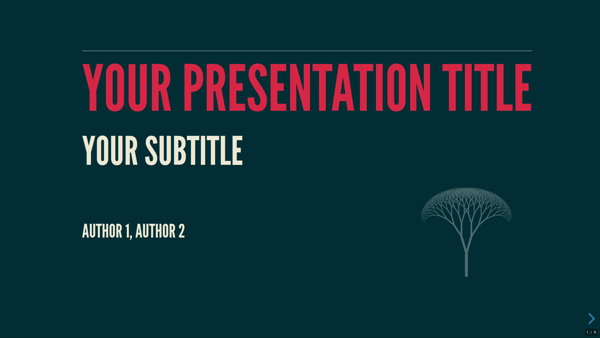
slide1 = Slide(center=True)
# Content for the title page
logo_url = "https://upload.wikimedia.org/wikipedia/commons/4/4d/Fractal_canopy.svg"
title_page_content = {
'title': 'Your presentation title',
'subtitle': 'Your subtitle',
'authors': 'Author 1, Author 2',
'logo': logo_url
}
# Styles for the title page content in the same order as content
styles = [
{'color': '#e63946', 'class': 'r-fit-text border-top'}, # title
{}, # subtitle style by default
{}, # authors style by default
{'filter': 'invert(100%) opacity(30%)'}, # logo
]
# Add the title page to the slide
slide1.add_title_page(title_page_content, styles)
You can pass CSS styles and classes as kwargs. For example, in the code below,
the add_title method takes a dictionary kwarg styles containing :
- one or several CSS styles as key : values
- and class as a unique key:
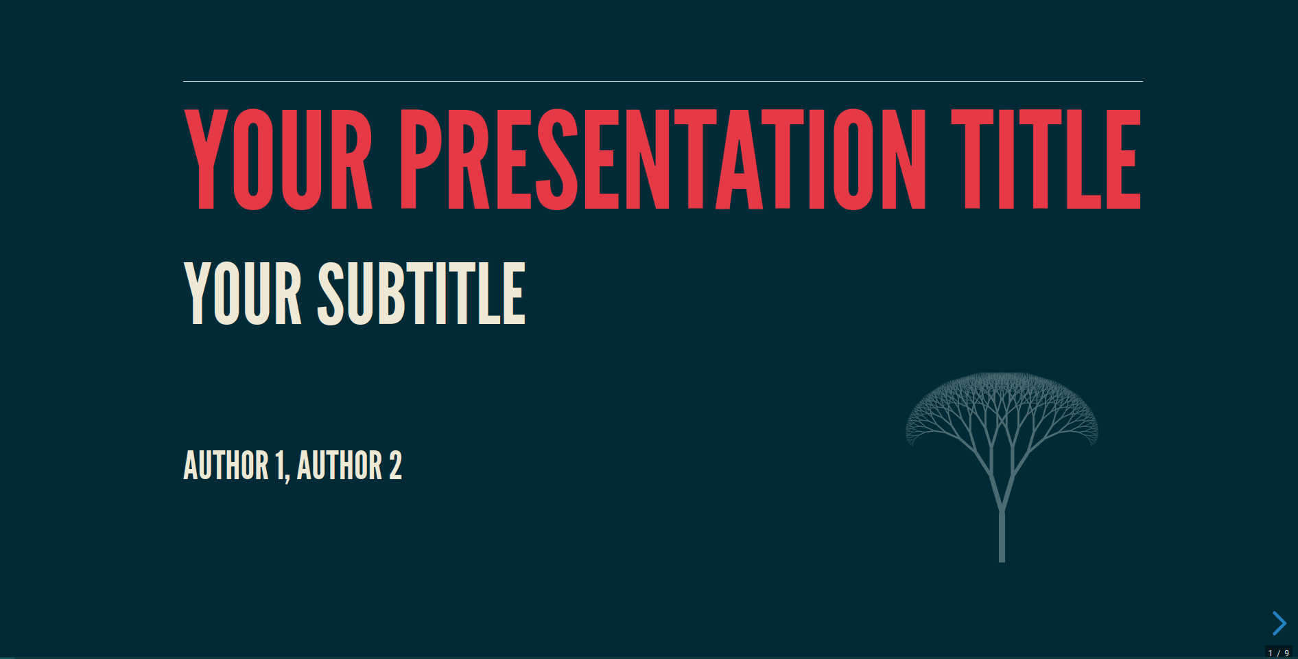
Split title page layout
As an alternative to the classic title page, you can create a split layout with the title content on one side and custom content (logo, image, chart) on the other side using add_split_title_page():
# Create a slide with split title page layout
slide1b = Slide(center=True)

# Content for the split title page
split_title_content = {
    'title': 'Your presentation title',
    'subtitle': 'Your subtitle',
    'authors': 'Author 1, Author 2',
}

# Styles for the title elements
title_styles = [
    {'color': '#e63946', 'font-weight': 'bold', 'font-size': '60px'},  # title
    {'color': '#457b9d', 'font-size': '40px'},  # subtitle
    {'color': '#457b9d', 'font-size': '25px'},  # authors
]

# Style for the title column
title_column_style = {
    'background-color': '#1d3557',
    'color': '#f1faee',
    'padding': '40px',
    'border-radius': '10px 0 0 10px'
}

# Style for the custom content column
image_style = {
    'text-align': 'center',
    'padding': '30px',
    'background-color': '#e63946',
    'border-radius': '0 10px 10px 0'
}

# Add the split title page - title on left (8 cols), logo on right (4 cols)
slide1b.add_split_title_page(
    title_page_content=split_title_content,
    custom_content=logo_url,
    title_column_width=8,
    custom_column_width=4,
    title_page_class="split-intro",
    custom_content_style=image_style,
    title_styles=title_styles,
    title_column_style=title_column_style
)
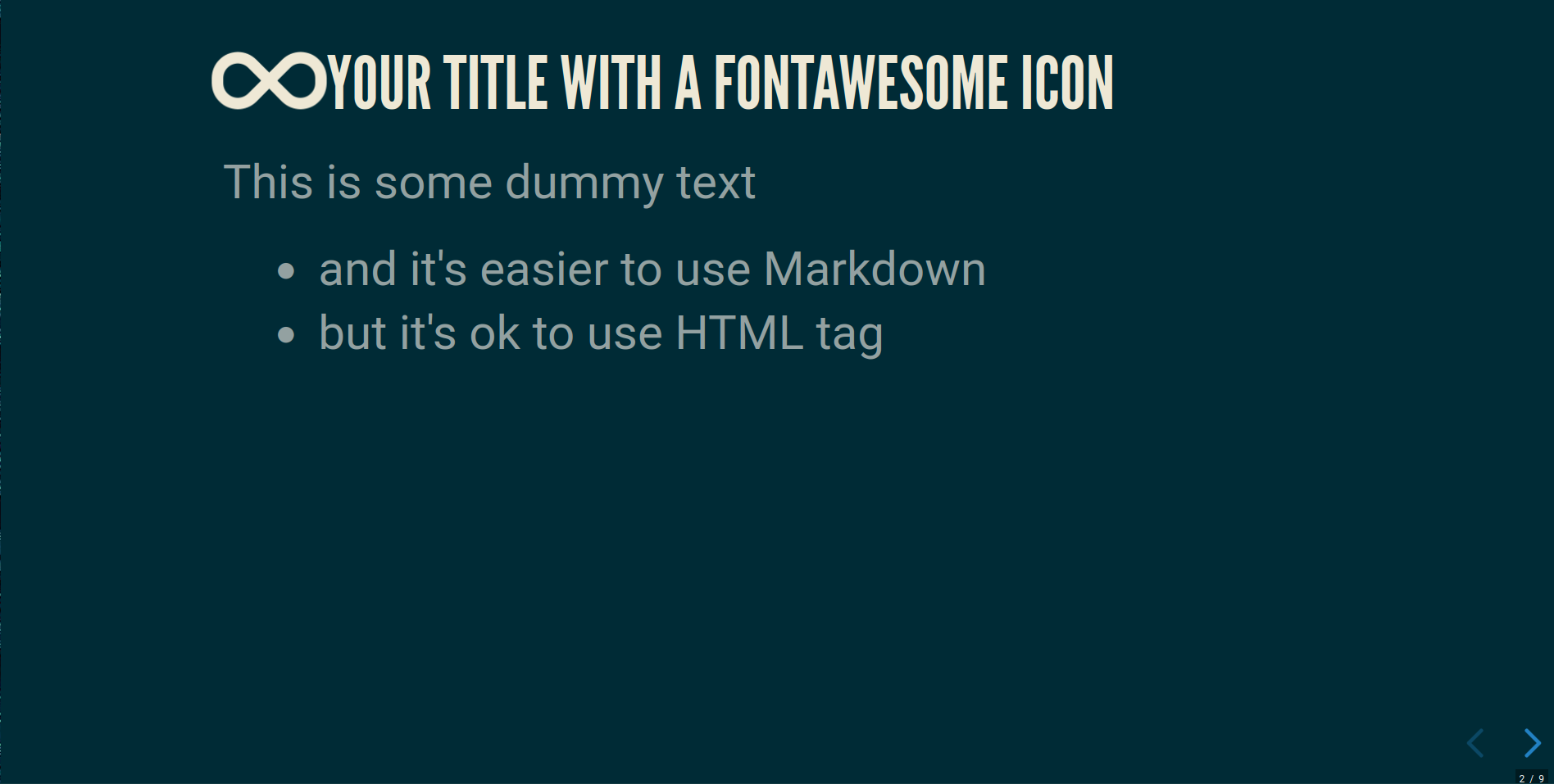
A simple text slide
Now, lets create a simple slide with a title and some content.
Markdown is more intuitive, so we will use it, but it's not mandatory.
# Create the second slide
slide2 = Slide()

# Add a title to the slide with a fontawesome icon
slide2.add_title("Your title with a fontawesome icon", icon="fas fa-infinity fa-beat")

# Create some text in markdown format
txt = markdown("""
This is some dummy text

- and it's easier to use Markdown
<ul><li>but it's ok to use HTML tag</li></ul>
""")

# Add the text to the slide in a new Bootstrap column with a width of 12 (default)
slide2.add_content([txt], columns=[12])
Note that for the add_title() method, Fontawesome icons can be added.
A two columns slide with text and image
Let's add two columns :
- the first with some text
- the second with an image
respysive-slide will try to find automatically the content type (txt, image, chart from json).
You only have to pass the content list with the add_content() method
# Create a new slide
slide3 = Slide()
text = markdown("""
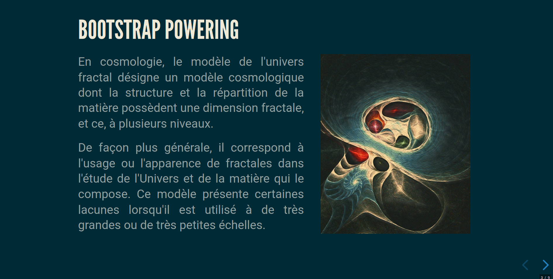
En cosmologie, le modèle de l'univers fractal désigne un modèle cosmologique
dont la structure et la répartition de la matière possèdent une dimension fractale,
et ce, à plusieurs niveaux.
De façon plus générale, il correspond à l'usage ou
l'apparence de fractales dans l'étude de l'Univers et de la matière qui le compose.
Ce modèle présente certaines lacunes lorsqu'il est utilisé à de très grandes ou de
très petites échelles.
""")
# Add image url
url = "./assets/img/Univers_Fractal_J.H..jpg"
# Add title to slide
slide3.add_title("Bootstrap powering")
# Add styles to slide
css_txt = [
{'font-size': '70%', 'text-align': 'justify', 'class': 'bg-warning'}, # text style
None # url style is mandatory even it is None
]
# Add content to slide, where text and url are added to the slide with 7 and 5 columns respectively
# css_txt is added as styles
slide3.add_content([text, url], columns=[7, 5], styles=css_txt)
Note that class can include Reveal.js fragments for step-by-step content reveal.
Plotly, Altair and Matplotlib
Plotly, Altair or Matplotlib graphs can be easily added with add_content(). Interactivity
is fully functional for Plotly and Altair.
slide4 = Slide()
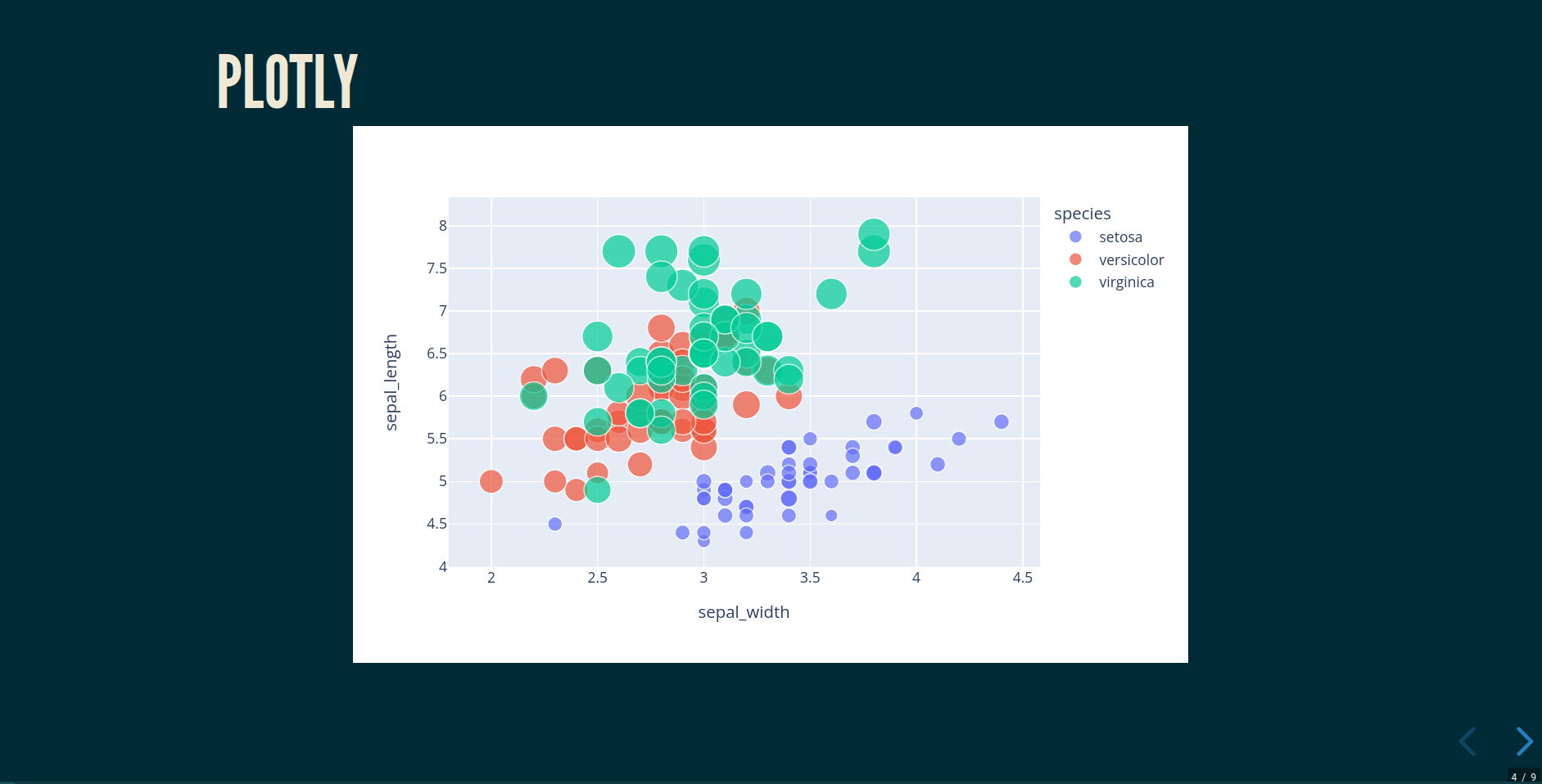
slide4.add_title("Plotly")
# import plotly express for creating scatter plot
import plotly.express as px
# load iris data
df = px.data.iris()
# create scatter plot
fig = px.scatter(df, x="sepal_width", y="sepal_length",
color="species", size="petal_length", hover_data=["petal_width"])
# update layout
fig.update_layout(autosize=True)
# Export the figure to json format
j = fig.to_json()
# apply css to the figure
css_txt = [{'class': 'stretch'}]
# add the scatter plot to the slide
slide4.add_content([j], columns=[12], styles=css_txt)
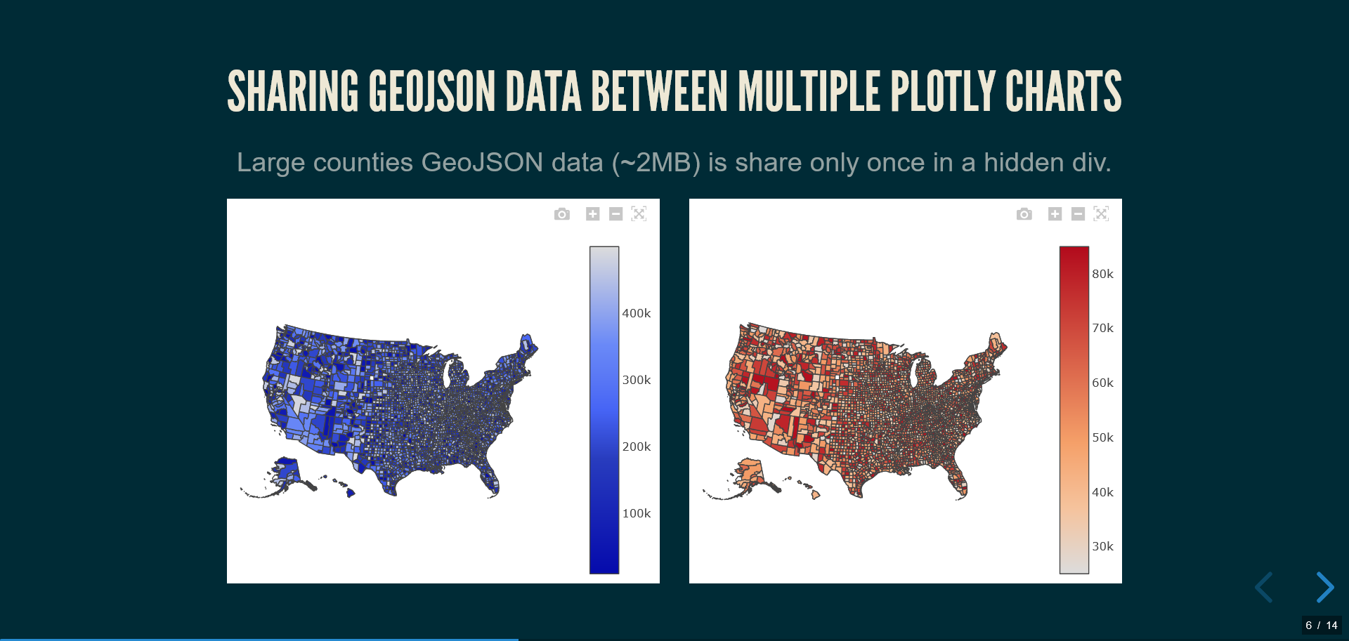
Sharing GeoJSON data between multiple Plotly charts
You can optimize performance by sharing large data (like GeoJSON) between multiple charts across the entire presentation.
Simple example:
# Add shared data once
p.add_global_geojson("my_data", geojson_dict)
# Use in multiple charts with shared_data_ids parameter
slide.add_content([chart1, chart2],
                  columns=[6, 6],
                  shared_data_ids=["my_data", "my_data"])
Complete example:
from respysive import Presentation, Slide

# Create presentation
p = Presentation()

# Load GeoJSON data
from urllib.request import urlopen
import json
with urlopen('https://raw.githubusercontent.com/plotly/datasets/master/geojson-counties-fips.json') as response:
    counties = json.load(response)

# Load unemployment data
import pandas as pd
df_counties = pd.read_csv("https://raw.githubusercontent.com/plotly/datasets/master/fips-unemp-16.csv", dtype={"fips": str})

# Add additional columns with pandas
import random
random.seed(42)
df_counties['population'] = [random.randint(10000, 500000) for _ in range(len(df_counties))]
df_counties['income'] = [random.randint(25000, 85000) for _ in range(len(df_counties))]
# Add area data for density calculation
df_counties['area_sq_miles'] = [random.randint(200, 2000) for _ in range(len(df_counties))]
df_counties['density'] = (df_counties['population'] / df_counties['area_sq_miles']).round(1)

# Add global geojson data to presentation
p.add_global_geojson("us_counties", counties)

slide_maps = Slide()
slide_maps.add_title("Sharing geojson data between multiple plotly charts", **{'class': 'r-fit-text'})

# Add context text
context_text = """
Counties geojson data (~2MB) is shared across the presentation
"""

css_txt = [{'text-align': 'center', 'font-size': "70%"}]

slide_maps.add_content([context_text], columns=[12], styles=css_txt)

# Create population density map
population_config = {
    "data": [{
        "type": "choropleth",
        "locations": df_counties['fips'].tolist(),
        "z": df_counties['density'].tolist(),
        "colorscale": "Blues",
        "colorbar": {
            "title": "Density<br>(per sq mi)",
            "thickness": 15,
            "len": 0.7
        },
        "hovertemplate": (
            "<b>County {text}</b><br>" +
            "Population: %{customdata[0]:,.0f}<br>" +
            "Area: %{customdata[1]:,.0f} sq mi<br>" +
            "Density: <b>%{z:.1f} per sq mi</b>" +
            "<extra></extra>"
        ),
        "text": df_counties['fips'].tolist(),
        "customdata": list(zip(df_counties['population'], df_counties['area_sq_miles']))
    }],
    "layout": {
        "geo": {
            "projection": {"type": "albers usa"},
            "scope": "usa",
            "showlakes": True,
            "lakecolor": "lightblue"
        },
        "title": {
            "text": "Population Density by County (Random Data)",
            "x": 0.5,
            "xanchor": "center",
            "font": {"size": 16}
        },
        "margin": {"r":10,"t":50,"l":10,"b":10}
    }
}

# Create choropleth map for income
income_config = {
    "data": [{
        "type": "choroplethmap",
        "locations": df_counties['fips'].tolist(),
        "z": df_counties['income'].tolist(),
        "colorscale": [
            [0.0, "#ffffb2"],
            [0.2, "#fed976"],
            [0.4, "#feb24c"],
            [0.6, "#fd8d3c"],
            [0.8, "#f03b20"],
            [1.0, "#bd0026"]
        ],
        "colorbar": {
            "title": {
                "text": "Median Income ($)",
                "font": {"size": 14, "family": "Arial Black"}
            },
            "thickness": 20,
            "len": 0.8,
            "x": 1.02,
            "tickmode": "array",
            "tickvals": [25000, 40000, 55000, 70000, 85000],
            "ticktext": ["$25K", "$40K", "$55K", "$70K", "$85K"],
            "tickfont": {"size": 11}
        },
        "hovertemplate": (
            "<b>County FIPS: %{location}</b><br>" +
            "Median Income: <b>$%{z:,.0f}</b><br>" +
            "Population: <b>%{customdata:,.0f}</b>" +
            "<extra></extra>"
        ),
        "customdata": df_counties['population'].tolist(),
        "marker": {
            "line": {"color": "white", "width": 0.5},
            "opacity": 0.9
        }
    }],
    "layout": {
        "map": {
            "style": "carto-positron",
            "zoom": 3.2,
            "center": {"lat": 38.0, "lon": -97.0}
        },
        "title": {
            "text": "Median Household Income by County (Random Data)",
            "x": 0.5,
            "xanchor": "center",
            "font": {
                "size": 18,
                "family": "Arial Black",
                "color": "#2E86AB"
            },
            "pad": {"t": 20}
        },
        "annotations": [{
            "text": "Data source: Simulated random data",
            "showarrow": False,
            "x": 0.99,
            "y": 0.01,
            "xref": "paper",
            "yref": "paper",
            "xanchor": "right",
            "yanchor": "bottom",
            "font": {"size": 10, "color": "gray"}
        }],
        "margin": {"r":80,"t":80,"l":20,"b":40},
        "paper_bgcolor": "rgba(248, 249, 250, 0.95)"
    }
}

# Add the two maps side by side using shared GeoJSON data
slide_maps.add_content(
    [population_config, income_config],
    columns=[6, 6],
    shared_data_ids=["us_counties", "us_counties"]
)
This approach stores the large counties GeoJSON data (~2MB) only once globally in the presentation. Multiple maps across any slides can then reference this shared data, avoiding duplication.
Compatible map types:
choropleth- Standard geographic choropleth mapschoroplethmap- Modern tile-based choropleth mapsscattermap/scattermapbox- Scatter plots on maps- Line plots on maps (using
scattermapwithmode: "lines")
Altair
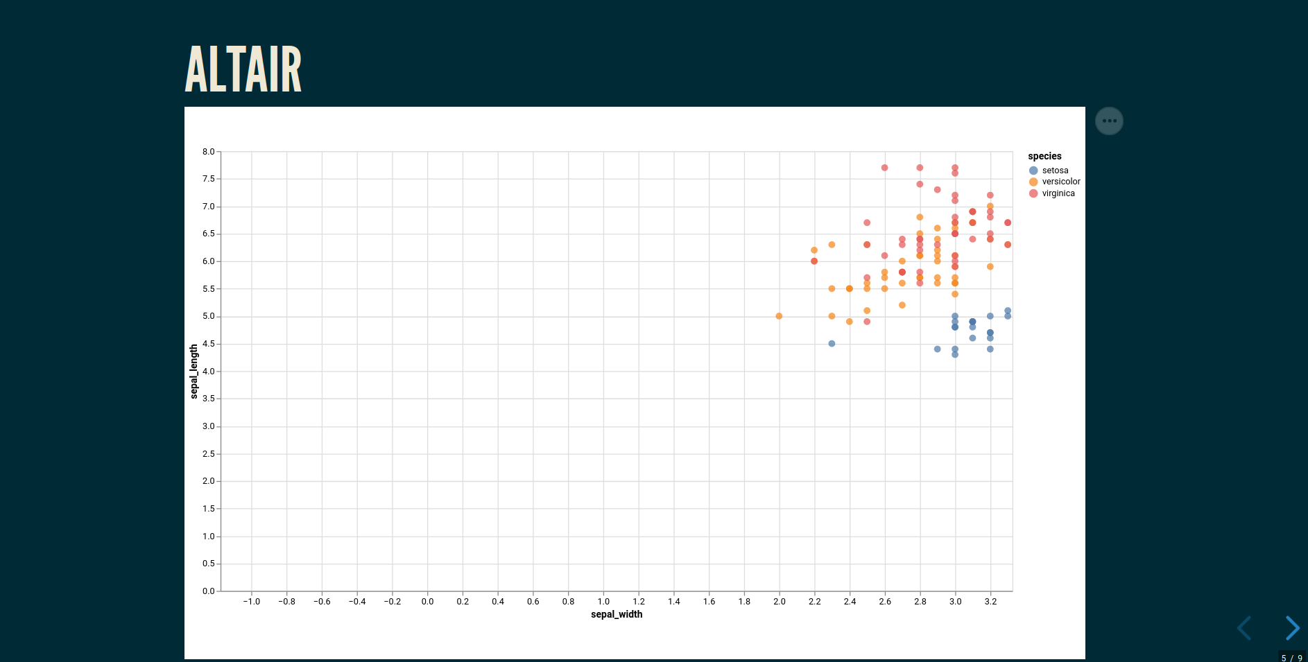
slide5 = Slide()
slide5.add_title("Altair")

# import altair for creating scatter plot
import altair as alt

source = px.data.iris()

# create scatter plot
chart = (
    alt.Chart(source)
    .mark_circle(size=60)
    .encode(
        x="sepal_width", y="sepal_length", color="species",
        tooltip=["species", "sepal_length", "sepal_width"],
    )
    .interactive()
    .properties(width=900, height=500)
)

# Export the figure to json format
j = chart.to_json()

# add the scatter plot to the slide
slide5.add_content([j], columns=[12])
Matplotlib fig are automatically converted to svg
slide5_fig = Slide()
slide5_fig.add_title("Matplotlib")

import numpy as np
import matplotlib.pyplot as plt

x = np.arange(0,4*np.pi-1,0.1)   # start,stop,step
y = np.sin(x)
z = np.cos(x)

plt.rcParams["figure.figsize"] = (8, 5)
fig, ax = plt.subplots()
plt.plot(x,y,x,z)
plt.xlabel('x values')
plt.title('sin and cos ')
plt.legend(['sin(x)', 'cos(x)'])

# add the  plot to the slide
slide5_fig.add_content([fig], columns=[12])
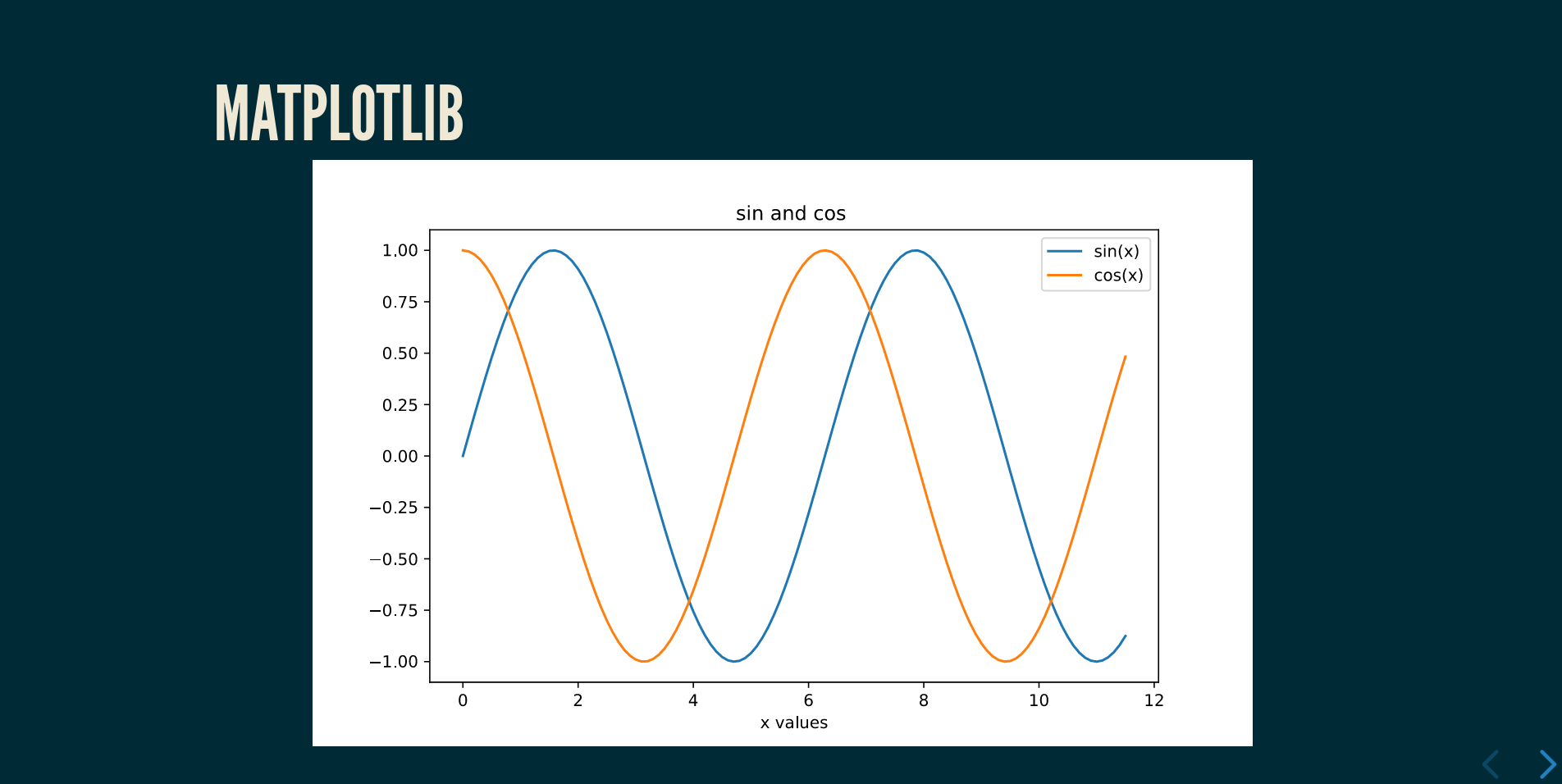
It is highly recommended to set chart's width and height manually
LaTeX support
You can use LaTeX mathematical expressions in your slides. The package automatically detects and processes LaTeX syntax:
slide6 = Slide()
slide6.add_title("Mathematical Equations")

# Text with LaTeX expressions
math_content = """
The Gaussian function $f(x) = e^{-x^2}$ or in display mode:

$$f(x) = e^{-x^2}$$
"""

slide6.add_content([math_content], columns=[12])
The LaTeX processing is automatic when you include $ or $$ delimiters in your text content.
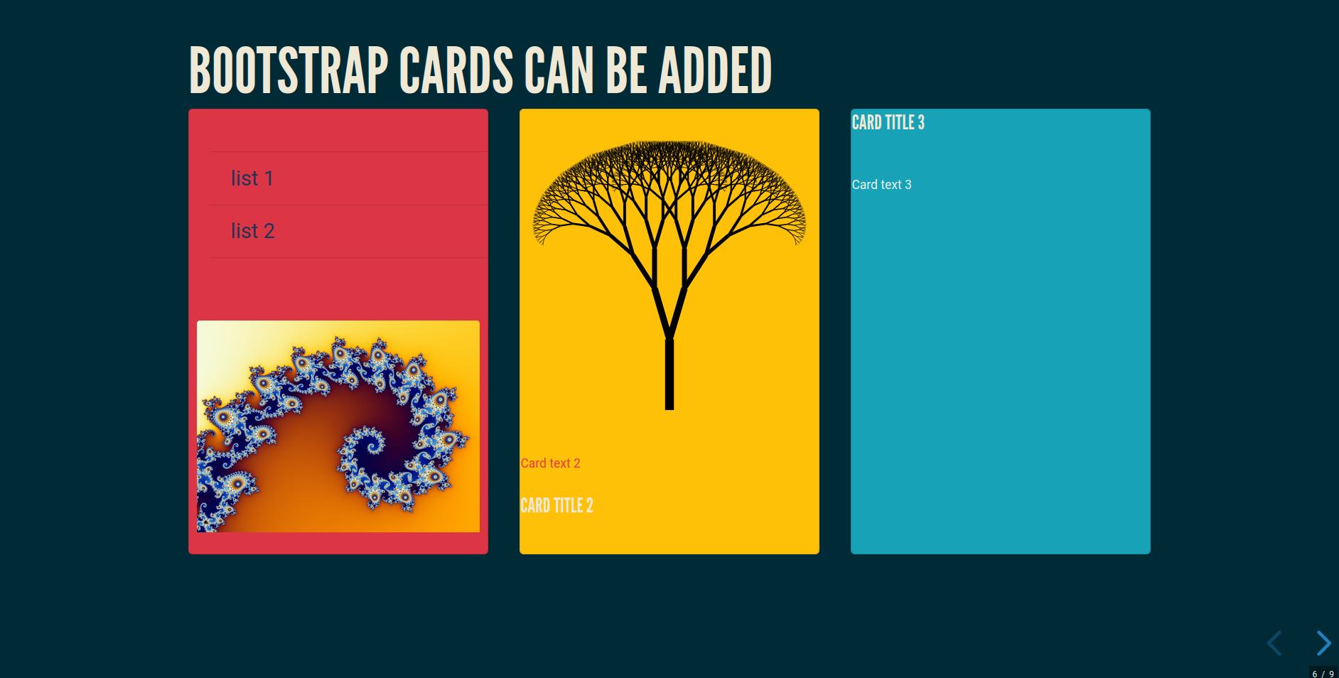
Bootstrap cards
Bootstrap Cards can also be added with add_card() method.
slide7 = Slide()

# card 1 content
txt_card1 = markdown("""
- list 1
- list 2

""")

# card 1 image
univ_url = "https://upload.wikimedia.org/wikipedia/commons/b/b5/Mandel_zoom_04_seehorse_tail.jpg"

# list of cards. These orders will be the same on the HTML page
cards = [{'text': txt_card1, 'image': univ_url},  # Only text and image
         {'image': logo_url, 'text': "Card text 2", 'title': "Card Title 2", },  # Image, text and title
         {'title': "Card Title 3", 'text': "Card text 3"}]  # Title and text

# styles for each cards
styles_list = [{'font-size': '20px', 'color': '#1d3557', 'class': 'bg-danger'},
               {'font-size': '20px', 'color': '#e63946', 'class': 'bg-warning'},
               {'font-size': '20px', 'color': '#f1faee', 'class': 'bg-info'}]

# add title and card to slide
slide7.add_title("Bootstrap cards can be added")
slide7.add_card(cards, styles_list)
Background image
Reveal.js Slide Backgrounds by passing a class data-background-* to
the Slide() method with a kwarg
bckgnd_url = "https://upload.wikimedia.org/wikipedia/commons/thumb/0/0a/Frost_patterns_2.jpg/1920px-Frost_patterns_2.jpg"

# Create a dictionary with slide kwargs
slide_kwargs = {
    'data-background-image': bckgnd_url,
    'data-background-size': 'cover',  # more options here : https://revealjs.com/backgrounds/
}

# Create a slide object with slide kwargs
slide8 = Slide(center=True, **slide_kwargs)

css_background = {"class": "text-center", "color": "#e63946", "background-color": "#f1faee"}
slide8.add_title("Image  background", **css_background)

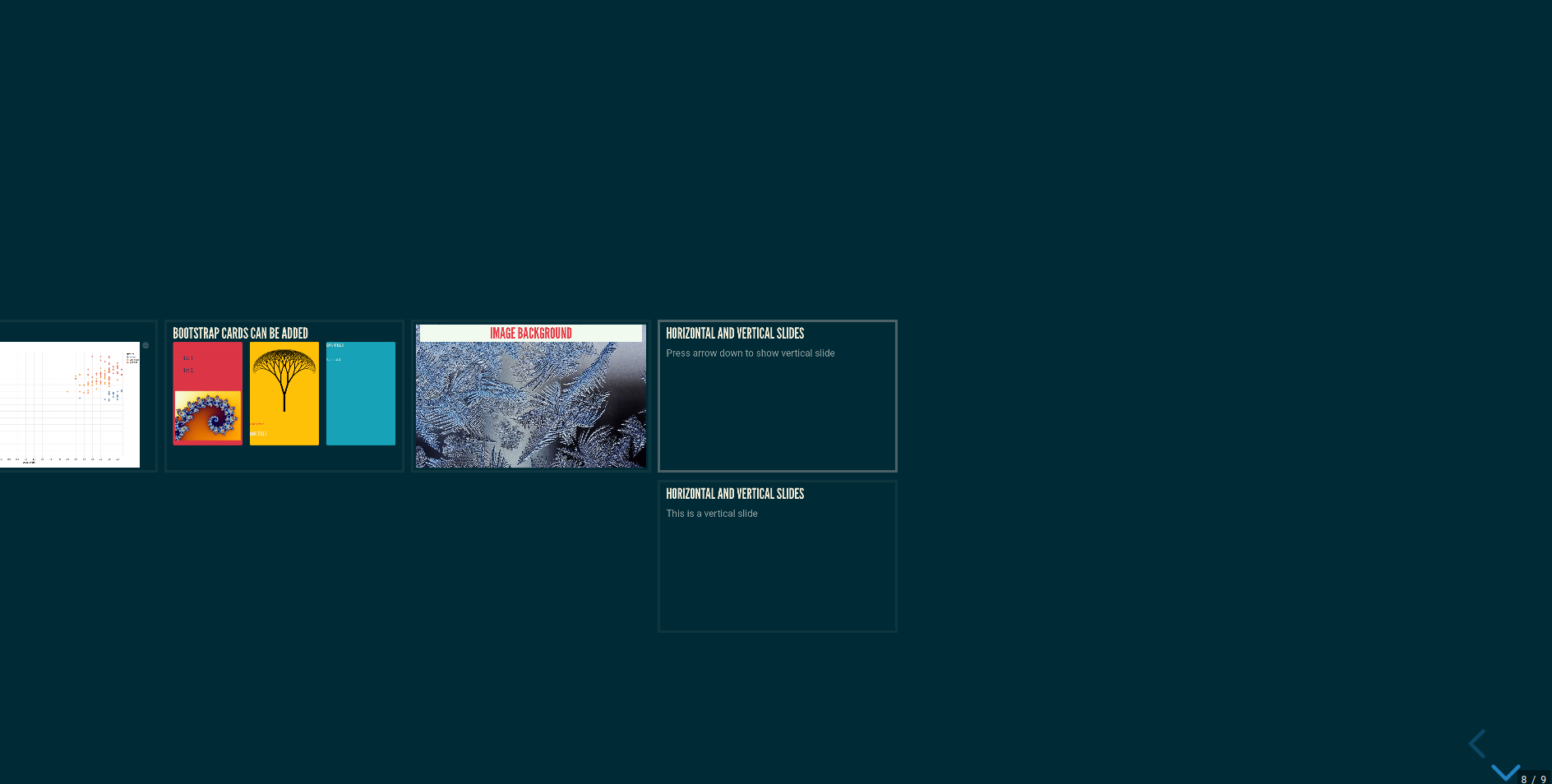
Vertical slides
You can add vertical slides. First, let's create slide 9 (horizontal one) and slide 10 (vertical one)
slide9 = Slide()
text = markdown("""Press arrow down to show vertical slide""")
slide9.add_title("Horizontal and vertical slides")
slide9.add_content([text])

slide10 = Slide(center=True)
slide10.add_title("Horizontal and vertical slides")
text = markdown("""This is a vertical slide""")
slide10.add_content([text])
They will be added as list in the next method to export your presentation
Speaker notes
You can add speaker notes to your slides which will be visible in the speaker view:
slide11 = Slide()
slide11.add_title("Speaker view")
text = markdown("""Press S for Speaker View""")

# Add speaker notes
speaker_notes = markdown("""
  <aside class="notes">
    This is a test for speaker view
  </aside>
""")

slide11.add_content([text])
slide11.add_content([speaker_notes])
Press 'S' during the presentation to open the speaker view with your notes.
Presentation rendering
Last step in rendering your Reveal.js presentation with respysive-slide as HTML
The Presentation.add_slide() method is used
# Adding slide to the presentation
p.add_slide([slide1, slide1b, slide2, slide3, slide4, slide_maps, slide5, slide5_fig, slide6, slide7, slide8, [slide9, slide10], slide11])

# Saving the presentation in HTML format
p.save_html("readme_example.html")
As you can see, slides 9 and 10 are inside a list. That tells respysive-slide to create vertical slide
Different Reveal.js theme and parameters can be added :
p.save_html(file_name,
            theme="moon",
            width=960,
            height=600,
            minscale=0.2,
            maxscale=1.5,
            margin=0.1,
            custom_theme=None,  # If theme="custom", pass here the custom css url
            center=True,        # Vertical centering of slides (default: True)
            embedded=False)     # Embedded presentation mode (default: False)
Vertical centering and layout options
center=True(default): Slides are vertically centered on screen based on contentcenter=False: Slides remain at fixed height, content aligns to top - useful for presentations with lots of contentembedded=True: Presentation adapts to its container size - useful for embedding in web pagesembedded=False(default): Presentation covers full browser viewport
PDF export
The slide can be exported with the classic Reveal.js method.
Just add ?print-pdf at the end of the url and open the in-browser print dialog : https://raw.githack.com/fbxyz/respysive-slide/master/readme_example.html?print-pdf .
Best results are obtained with Chrome or Chromium
Future features
- add method for speaker view
- offline presentation
- prettify the final rendering
Release history Release notifications | RSS feed


Download files
Download the file for your platform. If you're not sure which to choose, learn more about installing packages.
Source Distribution
Built Distribution
Filter files by name, interpreter, ABI, and platform.
If you're not sure about the file name format, learn more about wheel file names.
Copy a direct link to the current filters
File details
Details for the file respysive_slide-1.1.15.tar.gz.
File metadata
- Download URL: respysive_slide-1.1.15.tar.gz
- Upload date:
- Size: 26.8 kB
- Tags: Source
- Uploaded using Trusted Publishing? No
- Uploaded via: twine/6.1.0 CPython/3.13.5
File hashes
| Algorithm | Hash digest | |
|---|---|---|
| SHA256 |
1923daa9e3fd242f2430459f9356dd09fc0eb3d1e8034de65714959b14316880
|
|
| MD5 |
17452a22111bccdf9a0610473718b556
|
|
| BLAKE2b-256 |
7e26d9a6a5fa84c50ea0dc2dde01c3bccc29fcde74196bd98919c4cf1b4570af
|
File details
Details for the file respysive_slide-1.1.15-py3-none-any.whl.
File metadata
- Download URL: respysive_slide-1.1.15-py3-none-any.whl
- Upload date:
- Size: 22.9 kB
- Tags: Python 3
- Uploaded using Trusted Publishing? No
- Uploaded via: twine/6.1.0 CPython/3.13.5
File hashes
| Algorithm | Hash digest | |
|---|---|---|
| SHA256 |
2847805e8f3291d912cf38f1b8baac43eae3c9a62729edf7d307202170c291c6
|
|
| MD5 |
59e592b7cf3b07428d9345b412b18030
|
|
| BLAKE2b-256 |
89d20dfdeb456adda2736e2a3e0ab4fff048859bf95cce7c202f5f221e84ddc8
|


