

ReynoldsFlow




ReynoldsFlow is a finite-volume Python solver for steady incompressible flow in thin gaps with contact and complex percolating geometry. It solves Cartesian and polar forms of the Reynolds equation, retains all boundary-spanning fluid components, assembles only active degrees of freedom, and reconstructs conservative face fluxes from the same conductances used by the linear system.
The package is intended for rough-contact leakage calculations and related elliptic transport problems. Version 0.1.3 improves PETSc convergence checks and periodic pressure-gauge conditioning. Version 0.1.2 added fully periodic Cartesian pressure-gradient driving and compatibility with both scikit-sparse 0.4 and 0.5 while retaining the numerical conservation and solver diagnostics of the 0.1 series.
Mathematical model
For an isoviscous incompressible fluid with local gap g and pressure p, the
dimensionless Cartesian problem is
div(g³ grad(p)) = 0.
The Cartesian discretization is cell-centered on the unit square. Axis 0 is
the transport direction and axis 1 is periodic. By default, reservoir
pressures are applied at the west and east boundary faces. A representative
cell mode makes both axes periodic and prescribes the macroscopic pressure
gradient. Internal face conductivity is the harmonic mean of adjacent g³
values. Cells with g = 0 are impermeable; negative or non-finite gaps are
invalid input.
The polar solver discretizes the corresponding conservative annular operator
on (r, theta), with configurable radial pressures and periodic or symmetry
angular boundary conditions.
Main features
- Conservative Cartesian and polar finite-volume discretizations.
- Periodic connectivity analysis retaining every independent spanning channel.
- Compact sparse systems with one unknown per active percolating cell.
- Exact-size two-pass CSR assembly accelerated with Numba.
- Conservative face flux, total-flow integration, and conservation diagnostics.
- Direct and AMG-preconditioned iterative solvers with checked true residuals.
- Explicit errors for invalid input, unavailable backends, unknown solvers, breakdown, and non-convergence.
- Deterministic correctness and performance benchmarks.
Installation
The portable installation includes SciPy and PyAMG:
pip install reynoldsflow
Optional native backends can be installed separately:
pip install "reynoldsflow[pardiso]"   # pypardiso / oneMKL
pip install "reynoldsflow[cholesky]"  # scikit-sparse / CHOLMOD
pip install "reynoldsflow[petsc]"    # petsc4py binding
pip install "reynoldsflow[solvers]"  # request every optional Python binding
The Cholesky extra depends on scikit-sparse, which wraps the native
SuiteSparse/CHOLMOD library. If no compatible scikit-sparse wheel is
available, pip attempts a source build and requires the SuiteSparse development
headers and libraries to be installed first. In a Conda environment, the
recommended installation is:
conda install -c conda-forge scikit-sparse
pip install "reynoldsflow[cholesky]"
For a pip-based installation on Debian or Ubuntu, install
libsuitesparse-dev before running pip install "reynoldsflow[cholesky]".
On HPC systems, load the local SuiteSparse module or provide
SUITESPARSE_INCLUDE_DIR and SUITESPARSE_LIB_DIR to the build.
PETSc is also most reliable when its native stack and Python binding come from the same package manager. A tested Conda installation sequence is:
conda install -c conda-forge petsc petsc4py
pip install "reynoldsflow[petsc]"
The selected PETSc build must include Hypre for petsc-cg.hypre and MUMPS for
petsc-mumps; the standard conda-forge Linux build includes both. Keep PETSc
in a separate environment if another installed backend brings an incompatible
MPI runtime.
PETSc, MUMPS, Hypre, SuiteSparse, and oneMKL are native libraries. The PETSc
installation itself must have been built with the requested Hypre or MUMPS
support. Conda or a system/HPC package manager is often more reliable than
building these stacks through pip. Optional native backends are selected
explicitly; solver="auto" does not probe them because a broken MPI or MKL
installation may terminate below Python before a fallback is possible.
For plotting examples and development tools:
pip install "reynoldsflow[plot]"
pip install "reynoldsflow[dev]"
Quick start
This example computes flow around a circular impermeable inclusion:
import matplotlib.pyplot as plt
import numpy as np

from reynoldsflow import transport

n = 256
coordinate = (np.arange(n, dtype=float) + 0.5) / n
x, y = np.meshgrid(coordinate, coordinate, indexing="ij")
gaps = (np.hypot(x - 0.5, y - 0.5) > 0.2).astype(float)

filtered_gaps, pressure, flux = transport.solve_fluid_problem(
    gaps,
    solver="auto",
    p_west=0.0,
    p_east=1.0,
)

if pressure is not None:
    total_flux, conservation_error = transport.compute_total_flux(
        filtered_gaps, flux, n
    )
    print(f"Q = {total_flux:.8g}")
    print(f"relative conservation error = {conservation_error:.3e}")
    plt.imshow(pressure.T, origin="lower", extent=(0, 1, 0, 1))
    plt.colorbar(label="pressure")
    plt.show()
solve_fluid_problem returns (filtered_gaps, pressure, flux). A normal
non-percolating field returns (None, None, None); invalid data and solver
failures raise explicit exceptions. The default iterative tolerance is
rtol=1e-12.
For a Cartesian representative cell driven by
G = -mean(dp/dx), use:
filtered_gaps, pressure_fluctuation, flux = transport.solve_fluid_problem(
    gaps,
    solver="auto",
    boundary_mode="periodic",
    pressure_gradient=1.0,
)
Both axes are periodic in this mode and positive pressure_gradient drives
positive axis-0 flow. The returned pressure is the periodic fluctuation in
p = -G*x + pressure_fluctuation, normalized to zero mean separately on each
connected fluid component. Non-winding fluid pockets are retained and carry
zero net flux. If no component winds around axis 0, the solve returns the
normal (None, None, None) no-percolation result. p_west and p_east cannot
be combined with periodic mode. The same options are accepted by
prepare_fluid_problem for fixed-topology sequences.
For annular domains, use
reynoldsflow.transport_polar.solve_fluid_problem_polar.
Linear solvers
No backend is universally optimal. Sparse-direct methods are attractive as moderate-size references but exhibit fill-driven time and memory growth. Multigrid-preconditioned CG methods have higher setup costs and generally offer the better route to large systems.
| Solver string | Method and preconditioner | Dependency | Advantages | Limitations / best use |
|---|---|---|---|---|
auto |
CG + Ruge–Stuben AMG | SciPy, PyAMG | Portable and safe default; no native optional stack | Same implementation as scipy.amg-rs; slow on the largest rough-contact cases |
scipy.amg-rs |
CG + Ruge–Stuben AMG | SciPy, PyAMG | Low memory; portable; explicit iterations and residual | Reached 531 s at 5120² and exceeded the 6144² timeout |
scipy.amg-smooth_aggregation |
CG + smoothed-aggregation AMG | SciPy, PyAMG | Portable alternative; competitive on the largest release case | More hierarchy memory; performance is problem-dependent |
scipy-spsolve |
Sparse LU (SuperLU) | SciPy | Robust direct reference available in the base install | Used 23.1 GiB at 4096²; intended for small/moderate diagnostics |
cholesky |
Sparse Cholesky (CHOLMOD) | scikit-sparse, SuiteSparse | Very fast direct reference for the SPD operator | Native install; fill growth; performance depends strongly on BLAS |
pardiso |
Sparse Cholesky (oneMKL Pardiso) | pypardiso, oneMKL | Accurate direct solve; tunable shared-memory parallelism | Native runtime; thread-sensitive; factor memory grows rapidly |
petsc-cg.hypre |
CG + Hypre BoomerAMG | PETSc, Hypre | Few iterations; strongest large-scale option in current tests | PETSc/MPI installation and cold initialization cost |
petsc-cg.gamg |
CG + PETSc GAMG | PETSc | PETSc-native algebraic multigrid | Iteration count and setup are more problem-dependent than Hypre |
petsc-mumps |
Multifrontal direct solve | PETSc, MUMPS | Accurate direct reference inside PETSc | Used 16.8 GiB at 5120²; 6144² was killed under memory pressure |
Explicit native backends never silently fall back to another algorithm.
Reproducible v0.1.1 performance
The following figure replaces the legacy performance plots as the release
baseline. It uses the deterministic rough-contact case at 256², 512²,
1024², 2048², 4096², 5120², and 6144²; compact active-DOF systems;
rtol=1e-12; and one native thread. Every solver ran in an isolated process.
Runtime is the median of two fresh-solver, steady-process, end-to-end runs
after one cold run. It includes matrix assembly, preconditioner construction
or direct factorization, solution, and flux postprocessing. Peak RSS includes
imports, native runtime state, JIT state, the gap field, matrix, solver data,
and outputs.
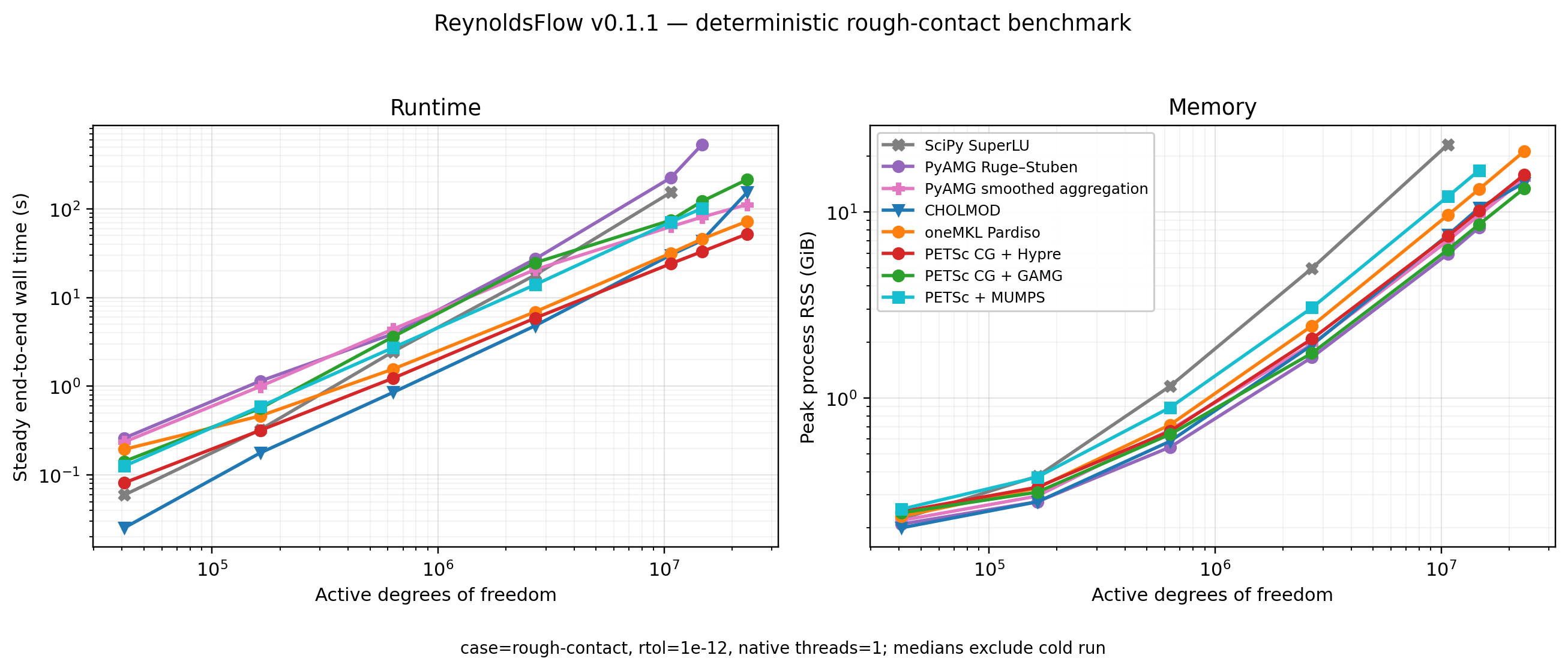
The 6144² case contained 23,301,121 active DOFs and 116,378,457 matrix
nonzeros. Five backends completed it:
| Solver | Steady end-to-end time (s) | Peak RSS (GiB) | Iterations |
|---|---|---|---|
petsc-cg.hypre |
52.18 | 15.85 | 16 |
pardiso |
72.40 | 21.22 | direct |
scipy.amg-smooth_aggregation |
111.90 | 15.05 | 26 |
cholesky |
153.52 | 14.36 | direct |
petsc-cg.gamg |
214.16 | 13.40 | 156 |
Curves stop at each backend's largest successful size. SuperLU stopped at
4096² (23.10 GiB; 5120² was projected above available RAM). MUMPS passed
5120² (101.26 s, 16.77 GiB) but received SIGKILL at 6144². Ruge–Stuben
passed 5120² (531.47 s, 8.26 GiB) but exceeded the 5400 s process timeout at
6144². Failed or unattempted points are not plotted as timings.
These values describe one matrix family and one binary environment; they are not universal backend rankings.
Benchmark host and numerical stack
- Machine: 13th Gen Intel Core i7-13700H, 14 physical cores / 20 logical CPUs, 32 GiB RAM, Linux 6.8 x86-64.
- Python 3.12.13; NumPy 2.4.2; SciPy 1.17.1; Numba 0.64.0; scikit-image 0.26.0; PyAMG 5.3.0.
- BLAS/LAPACK: conda-forge Netlib 3.11.0 for SciPy, CHOLMOD, PETSc, and MUMPS.
- Pardiso: pypardiso 0.4.7 with Intel oneMKL 2025.3.
- CHOLMOD: scikit-sparse 0.4.16 with SuiteSparse 7.10.1.
- PETSc stack: petsc4py 3.24.4, PETSc 3.24.5, OpenMPI 5.0.10, Hypre 3.1.0, and MUMPS 5.8.2; one MPI rank.
OMP_NUM_THREADS=MKL_NUM_THREADS=OPENBLAS_NUM_THREADS=1.
Commands and full stage definitions are documented in
benchmarks/README.md.
The compact-system and tolerance validation is summarized in
docs/performance-0.1.1.md.
Numerical validation
The test suite covers analytical Cartesian and polar solutions, matrix symmetry, conservative section fluxes, periodic connectivity, multiple spanning channels, compact/full-grid agreement, prepared-topology safeguards, solver diagnostics, and subprocess-isolated native backends.
python -m pytest -q
python -m pytest -q --run-backend tests/integration/test_optional_backends.py
Performance is never accepted without checking the true algebraic residual, finite pressure, total flow, and boundary-flux conservation.
Scope and limitations
- Steady, incompressible, isoviscous lubrication flow.
- Prescribed immobile gap field; no fluid–structure coupling.
- No cavitation, compressibility, inertia, or transient storage model.
- Cartesian public solves currently require square arrays.
- Native backend availability and performance depend on the local binary stack.
Illustrations
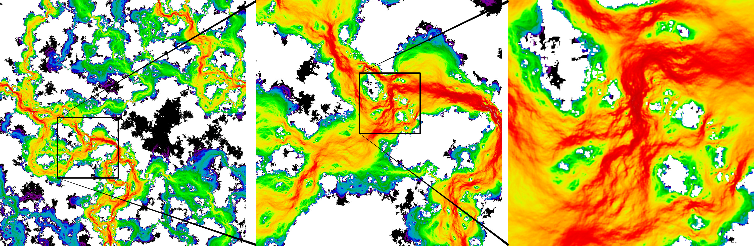
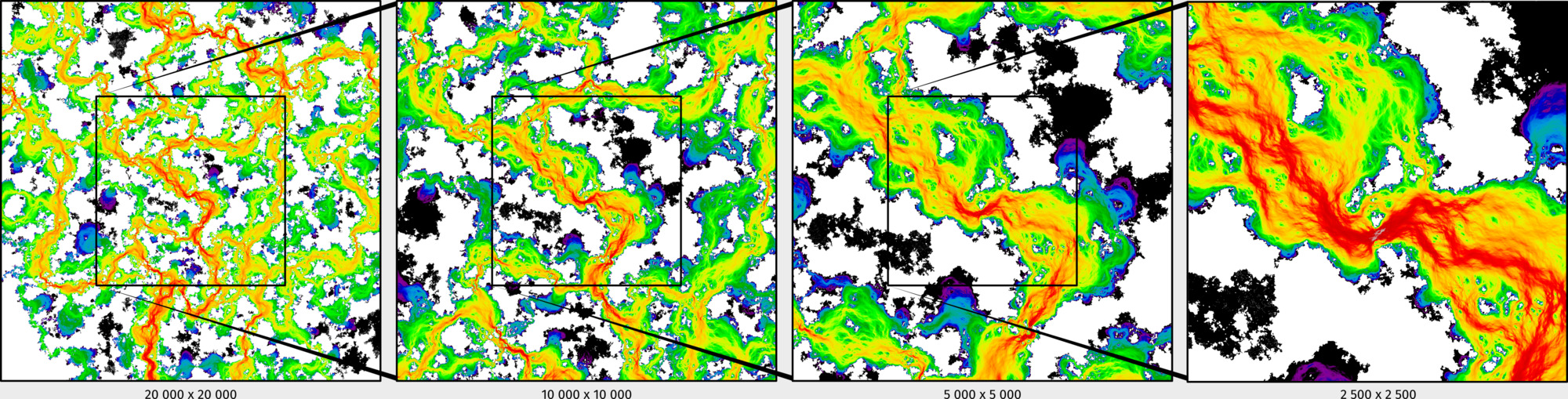
The following earlier large rough-contact simulations are retained as qualitative examples; they are not part of the v0.1.1 benchmark baseline.
Project information
Citation
If ReynoldsFlow contributes to scientific work, please cite the software using
the metadata in
CITATION.cff.
Credits
- Author: Vladislav A. Yastrebov, CNRS, Mines Paris – PSL, Centre des Matériaux.
- Development period: September 2025 – July 2026.
- License: BSD 3-Clause; see
LICENSE. - Repository: github.com/vyastreb/reynoldsflow.
- Changelog:
CHANGELOG.md.
AI-assisted development is acknowledged for Cursor and GitHub Copilot; ChatGPT 4o and 5; Claude 3.7, 4, and 4.5; and OpenAI Codex (GPT-5). Codex assisted with the numerical audit, regression tests, benchmark methodology, documentation, and 0.1-series release engineering. Scientific and numerical decisions and all generated code were reviewed by the author.
1 maintainer

Metadata
1 maintainer
Release files for reynoldsflow 0.1.3
For a detailed explanation of source distributions (sdists) and built distributions (wheels), please see the package formats documentation.
Source distribution (sdist)
| File | Size | Uploaded | |
|---|---|---|---|
| reynoldsflow-0.1.3.tar.gz | 478.4 kB | Details |
Built distribution (wheel)
| File | Interpreter | ABI | Platform | Reset |
|---|---|---|---|---|
| reynoldsflow-0.1.3-py3-none-any.whl | Python 3 | none | any | Details |
Total release size: 511.9 kB
Release files / reynoldsflow-0.1.3.tar.gz
| Download URL | reynoldsflow-0.1.3.tar.gz |
|---|---|
| Size | 478.4 kB |
| Tags | Source |
|
SHA-256 checksum How to use checksums |
ca22560fffff5ba6e313b0c9267b6cf8db6d10bd51a8c78b2a34cd77782a5d41
|
|
BLAKE2b-256 checksum How to use checksums |
b33a8a8f3284389947d45f84ecd12cddd83c957ac1a02767eea1c91d2f32b533
|
| Upload date | |
|
Uploaded using Trusted Publishing? What is trusted publishing? |
No |
| Uploaded via |
twine/7.0.0 CPython/3.10.12
|
Release files / reynoldsflow-0.1.3-py3-none-any.whl
| Download URL | reynoldsflow-0.1.3-py3-none-any.whl |
|---|---|
| Size | 33.6 kB |
| Tags | Python 3 |
|
SHA-256 checksum How to use checksums |
22a95f180989fdc9e933e47000cb0ce08850f34a135c24aafc8895a0b780d56e
|
|
BLAKE2b-256 checksum How to use checksums |
412cbaf2793b0b24de418685eb446ae7af60897364ea986c1d76a34f7f376ad0
|
| Upload date | |
|
Uploaded using Trusted Publishing? What is trusted publishing? |
No |
| Uploaded via |
twine/7.0.0 CPython/3.10.12
|














