1d lines, 3d maps

Project description
ridge_map

Ridge plots of ridges
A library for making ridge plots of... ridges. Choose a location, get an elevation map, and tinker with it to make something beautiful. Heavily inspired from Zach Cole's beautiful art, Jake Vanderplas' examples, and Joy Division's 1979 album "Unknown Pleasures".
Uses matplotlib, SRTM.py, numpy, and scikit-image (for lake detection).
Installation
Available on PyPI:
pip install ridge_map
Or live on the edge and install from github with
pip install git+https://github.com/colcarroll/ridge_map.git
You can also make a copy of this colab.
Want to help?
- I feel like I am missing something easy or obvious with lake/road/river/ocean detection, but what I've got gets me most of the way there. If you hack on the
RidgeMap.preprocessormethod and find something nice, I would love to hear about it! - Did you make a cool map? Open an issue with the code and I will add it to the examples.
Examples
The API allows you to download the data once, then edit the plot yourself, or allow the default processor to help you.
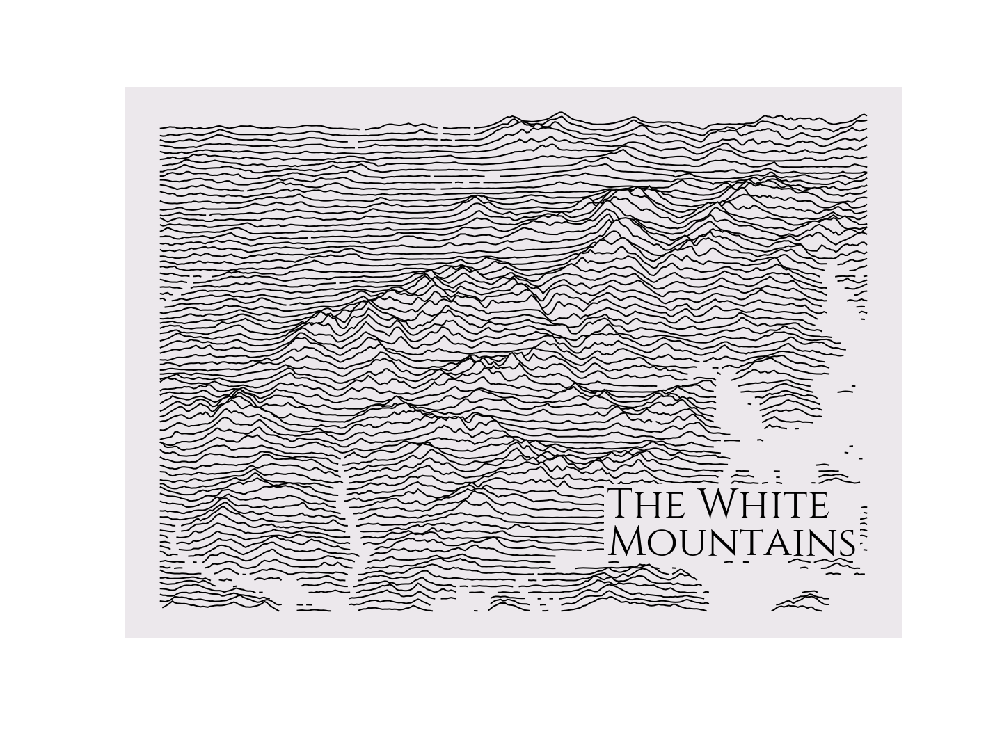
New Hampshire by default
Plotting with all the defaults should give you a map of my favorite mountains.
from ridge_map import RidgeMap

RidgeMap().plot_map()
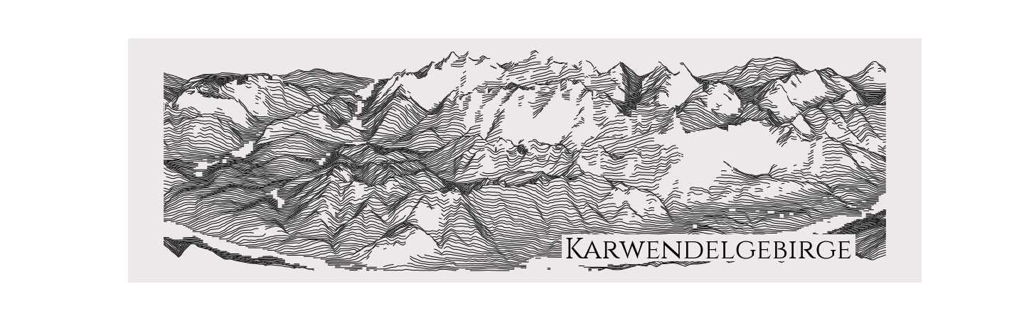
Download once and tweak settings
First you download the elevation data to get an array with shape
(num_lines, elevation_pts), then you can use the preprocessor
to automatically detect lakes, rivers, and oceans, and scale the elevations.
Finally, there are options to style the plot
rm = RidgeMap((11.098251,47.264786,11.695633,47.453630))
values = rm.get_elevation_data(num_lines=150)
values=rm.preprocess(
    values=values,
    lake_flatness=2,
    water_ntile=10,
    vertical_ratio=240)
rm.plot_map(values=values,
            label='Karwendelgebirge',
            label_y=0.1,
            label_x=0.55,
            label_size=40,
            linewidth=1)
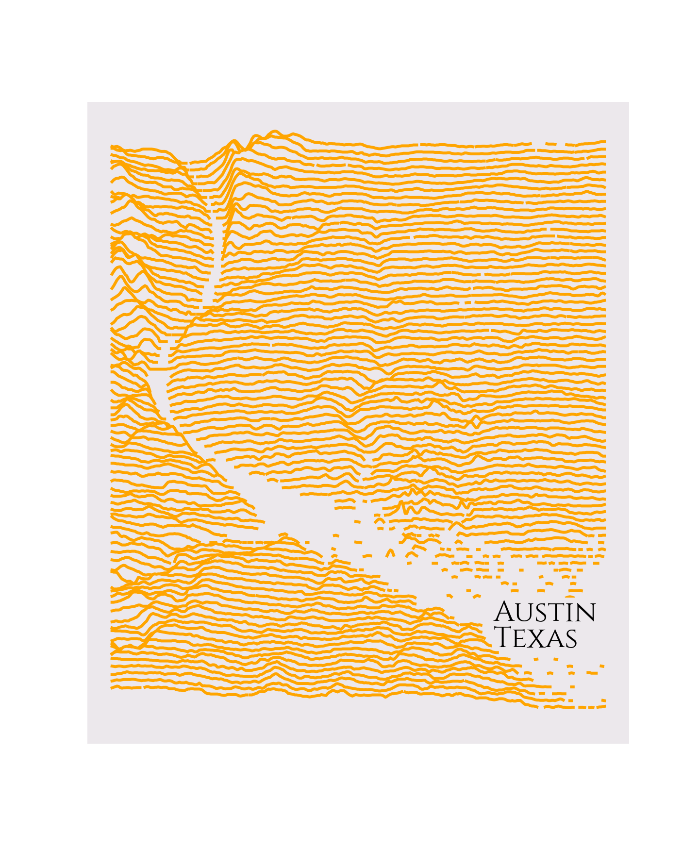
Plot with colors!
If you are plotting a town that is super into burnt orange for whatever reason, you can respect that choice.
rm = RidgeMap((-97.794285,30.232226,-97.710171,30.334509))
values = rm.get_elevation_data(num_lines=80)
rm.plot_map(values=rm.preprocess(values=values, water_ntile=12, vertical_ratio=40),
            label='Austin\nTexas',
            label_x=0.75,
            linewidth=6,
            line_color='orange')
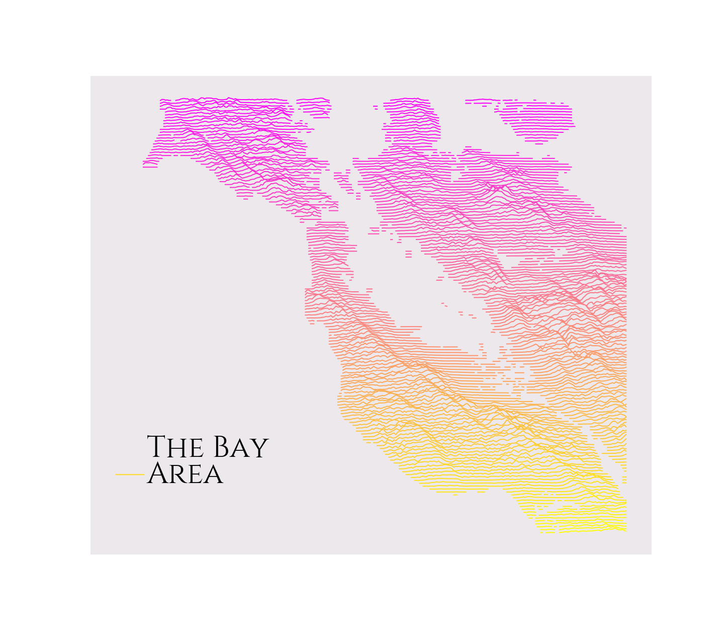
Plot with even more colors!
The line color accepts a matplotlib colormap, so really feel free to go to town.
rm = RidgeMap((-123.107300,36.820279,-121.519775,38.210130))
values = rm.get_elevation_data(num_lines=150)
rm.plot_map(values=rm.preprocess(values=values, lake_flatness=3, water_ntile=50, vertical_ratio=30),
            label='The Bay\nArea',
            label_x=0.1,
            line_color = plt.get_cmap('spring'))
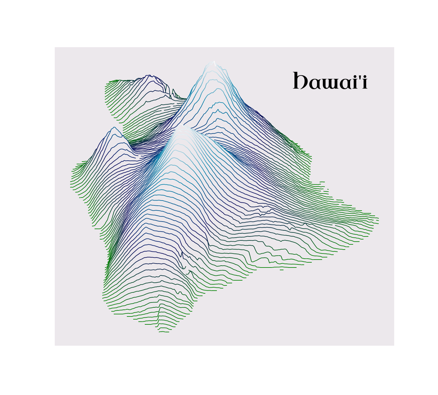
Plot with custom fonts and elevation colors!
You can find a good font from Google, and then get the path to the ttf file in the github repo.
If you pass a matplotlib colormap, you can specify kind="elevation" to color tops of mountains different from bottoms. ocean, gnuplot, and bone look nice.
from ridge_map import FontManager

font = FontManager('https://github.com/google/fonts/blob/main/ofl/uncialantiqua/UncialAntiqua-Regular.ttf?raw=true')
rm = RidgeMap((-156.250305,18.890695,-154.714966,20.275080), font=font.prop)

values = rm.get_elevation_data(num_lines=100)
rm.plot_map(values=rm.preprocess(values=values, lake_flatness=2, water_ntile=10, vertical_ratio=240),
            label="Hawai'i",
            label_y=0.85,
            label_x=0.7,
            label_size=60,
            linewidth=2,
            line_color=plt.get_cmap('ocean'),
            kind='elevation')
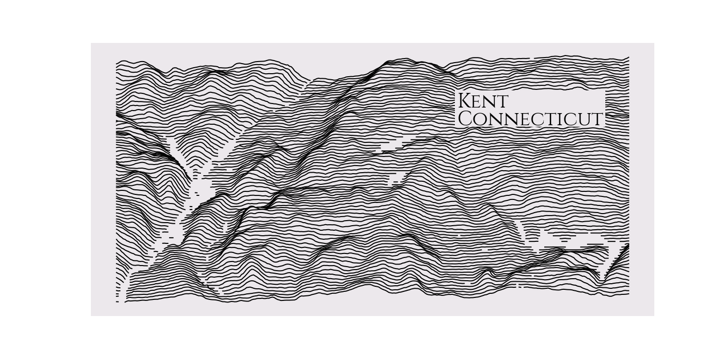
How do I find a bounding box?
I have been using this website. I find an area I like, draw a rectangle, then copy and paste the coordinates into the RidgeMap constructor.
rm = RidgeMap((-73.509693,41.678682,-73.342838,41.761581))
values = rm.get_elevation_data()
rm.plot_map(values=rm.preprocess(values=values, lake_flatness=2, water_ntile=2, vertical_ratio=60),
            label='Kent\nConnecticut',
            label_y=0.7,
            label_x=0.65,
            label_size=40)
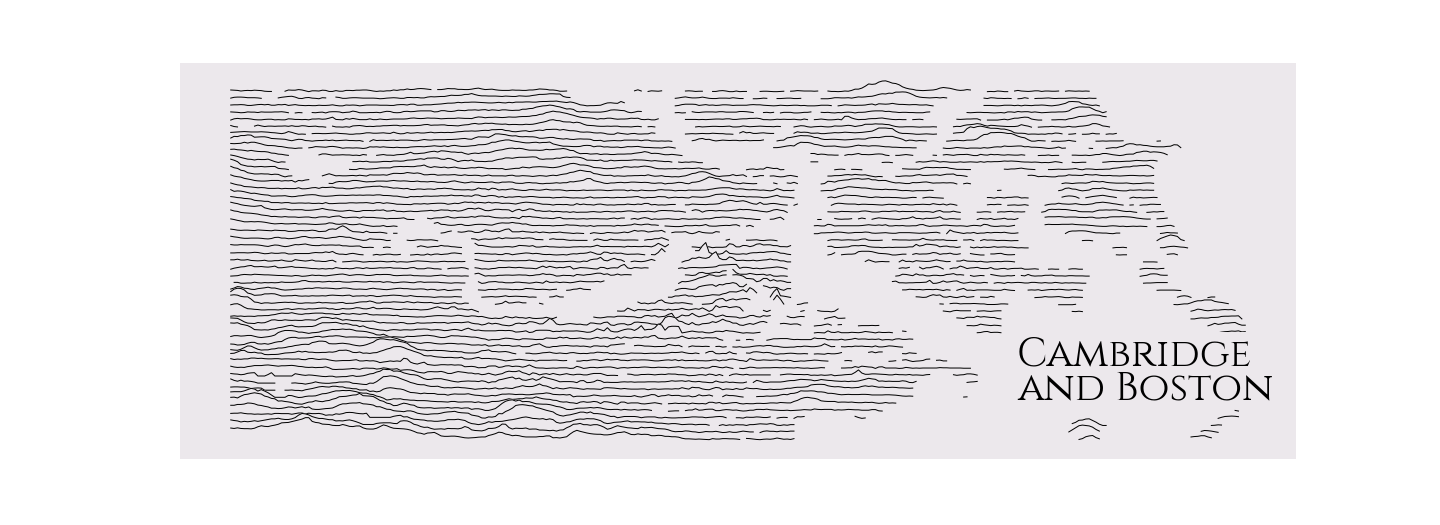
What about really flat areas?
You might really have to tune the water_ntile and lake_flatness to get the water right. You can set them to 0 if you do not want any water marked.
rm = RidgeMap((-71.167374,42.324286,-70.952454, 42.402672))
values = rm.get_elevation_data(num_lines=50)
rm.plot_map(values=rm.preprocess(values=values, lake_flatness=4, water_ntile=30, vertical_ratio=20),
            label='Cambridge\nand Boston',
            label_x=0.75,
            label_size=40,
            linewidth=1)
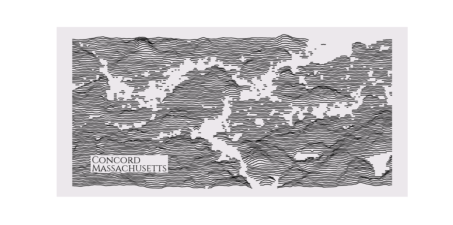
What about Walden Pond?
It is that pleasant kettle pond in the bottom right of this map, looking entirely comfortable with its place in Western writing and thought.
rm = RidgeMap((-71.418858,42.427511,-71.310024,42.481719))
values = rm.get_elevation_data(num_lines=100)
rm.plot_map(values=rm.preprocess(values=values, water_ntile=15, vertical_ratio=30),
            label='Concord\nMassachusetts',
            label_x=0.1,
            label_size=30)
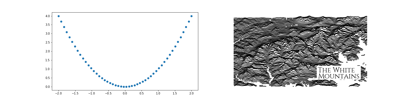
Do you play nicely with other matplotlib figures?
Of course! If you really want to put a stylized elevation map in a scientific plot you are making, I am not going to stop you, and will actually make it easier for you. Just pass an argument for ax to RidgeMap.plot_map.
import numpy as np
fig, axes = plt.subplots(ncols=2, figsize=(20, 5))
x = np.linspace(-2, 2)
y = x * x

axes[0].plot(x, y, 'o')

rm = RidgeMap()
rm.plot_map(label_size=24, background_color=(1, 1, 1), ax=axes[1])
User Examples
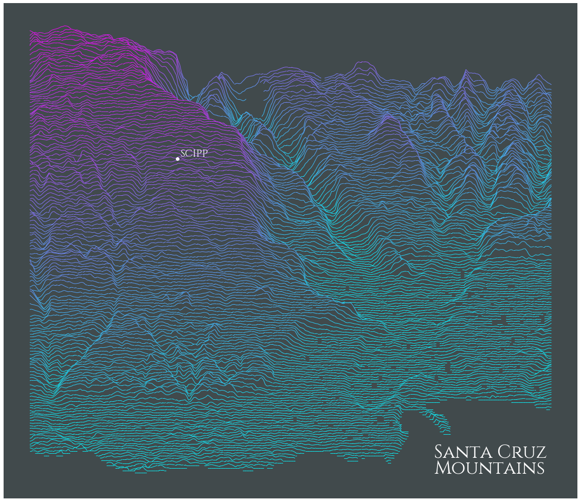
Annotating, changing background color, custom text
This example shows how to annotate a lat/long on the map, and updates the color of the label text to allow for a dark background. Thanks to kratsg for contributing.
import matplotlib
import matplotlib.pyplot as plt
import numpy as np

bgcolor = np.array([65,74,76])/255.

scipp = (-122.060510, 36.998776)
rm = RidgeMap((-122.087116,36.945365,-121.999226,37.023250))
scipp_coords = ((scipp[0] - rm.longs[0])/(rm.longs[1] - rm.longs[0]),(scipp[1] - rm.lats[0])/(rm.lats[1] - rm.lats[0]))

values = rm.get_elevation_data(num_lines=150)
ridges = rm.plot_map(values=rm.preprocess(values=values,
                                          lake_flatness=1,
                                          water_ntile=0,
                                          vertical_ratio=240),
            label='Santa Cruz\nMountains',
            label_x=0.75,
            label_y=0.05,
            label_size=36,
            kind='elevation',
            linewidth=1,
            background_color=bgcolor,
            line_color = plt.get_cmap('cool'))

# Bit of a hack to update the text label color
for child in ridges.get_children():
    if isinstance(child, matplotlib.text.Text) and 'Santa Cruz' in child._text:
        label_artist = child
        break
label_artist.set_color('white')

ridges.text(scipp_coords[0]+0.005, scipp_coords[1]+0.005, 'SCIPP',
            fontproperties=rm.font,
            size=20,
            color="white",
            transform=ridges.transAxes,
            verticalalignment="bottom",
            zorder=len(values)+10)

ridges.plot(*scipp_coords, 'o',
            color='white',
            transform=ridges.transAxes,
            ms=6,
            zorder=len(values)+10)
Elevation Data
Elevation data used by ridge_map comes from NASA's Shuttle Radar Topography Mission (SRTM), high resolution topographic data collected in 2000, and released in 2015. SRTM data are sampled at a resolution of 1 arc-second (about 30 meters). SRTM data is provided to ridge_map via the python package SRTM.py (link). SRTM data is not available for latitudes greater than N 60° or less than S 60°:


Download files
Download the file for your platform. If you're not sure which to choose, learn more about installing packages.
Source Distribution
Built Distribution
Filter files by name, interpreter, ABI, and platform.
If you're not sure about the file name format, learn more about wheel file names.
Copy a direct link to the current filters
File details
Details for the file ridge_map-0.0.6.tar.gz.
File metadata
- Download URL: ridge_map-0.0.6.tar.gz
- Upload date:
- Size: 13.5 kB
- Tags: Source
- Uploaded using Trusted Publishing? No
- Uploaded via: twine/6.0.1 CPython/3.11.11
File hashes
| Algorithm | Hash digest | |
|---|---|---|
| SHA256 |
126aa8873677276765283ae8d6d5100a161a4cfa9d24c2f014c105b623e40ddc
|
|
| MD5 |
10a4bb0e1fb40b698cab8e6b76748dba
|
|
| BLAKE2b-256 |
1d5b6fcf6bdd0264dee3066000532bc49998366646830dc28b85e74e25582598
|
File details
Details for the file ridge_map-0.0.6-py3-none-any.whl.
File metadata
- Download URL: ridge_map-0.0.6-py3-none-any.whl
- Upload date:
- Size: 10.1 kB
- Tags: Python 3
- Uploaded using Trusted Publishing? No
- Uploaded via: twine/6.0.1 CPython/3.11.11
File hashes
| Algorithm | Hash digest | |
|---|---|---|
| SHA256 |
ba8eeafea518283f1b2bfb385b66b38a9808a96b57b4ceb8af03ca81928f8171
|
|
| MD5 |
4a48fcc1ca0848ebbf238022287952ef
|
|
| BLAKE2b-256 |
1eb87c12553463553241971fa4798fb18a737ede520fe95f3f66a0f2bbfa8bc0
|


