Extreme value models for applications in energy procurement

Project description
riskmodels: a library for univariate and bivariate extreme value analysis (and applications to energy procurement)


This library focuses on extreme value models for risk analysis in one and two dimensions. MLE-based and Bayesian generalised Pareto tail models are available for one-dimensional data, while for two-dimensional data, logistic and Gaussian (MLE-based) extremal dependence models are also available. Logistic models are appropriate for data whose extremal occurrences are strongly associated, while a Gaussian model offer an asymptotically independent, but still parametric, copula.
The powersys submodule offers utilities for applications in energy procurement, with functionality to model available conventional generation (ACG) as well as to calculate loss of load expectation (LOLE) and expected energy unserved (EEU) indices on a wide set of models; efficient parallel time series based simulation for univariate and bivariate power surpluses is also available.
Requirements
Python >= 3.7
Installation
pip install riskmodels
API docs
https://nestorsag.github.io/riskmodels/
Quickstart
Because this library grew from research in energy procurement, this example is related to that but the univariate and bivariate modules are quite general and can be applied to any kind of data. The following example analyses the co-occurrence of high demand net of renewables (this is, demand minus intermittent generation such as wind and solar) in Great Britain's and Denmark's power systems. This can be done to value interconnection in the context of security of supply analysis, for example.
Table of contents
Quickstart - extreme value modelling
Quickstart - energy procurement modelling
Getting the data
The data for this example corresponds roughly to peak (winter) season of 2017-2018, and is openly available online but has to be put together from different places, namely Energinet's API, renewables.ninja, and NGESO's website.
from urllib.request import Request, urlopen
import urllib.parse
import requests

from datetime import timedelta

import pandas as pd
import numpy as np
import matplotlib.pyplot as plt

def fetch_data() -> pd.DataFrame:
  """Fetch data from different sources to reconstruct demand net of wind time series
  in Great Britain and Denmark.

  Returns:
      pd.DataFrame: Cleaned data
  """
  def fetch_gb_data():
    rn_prefix = "https://www.renewables.ninja/country_downloads"
    wind_url = f"{rn_prefix}/GB/ninja_wind_country_GB_current-merra-2_corrected.csv"
    wind_capacity = 13150
    #
    ngeso_prefix = "https://data.nationalgrideso.com/backend/dataset/8f2fe0af-871c-488d-8bad-960426f24601/resource"
    demand_urls = [
      f"{ngeso_prefix}/2f0f75b8-39c5-46ff-a914-ae38088ed022/download/demanddata_2017.csv",
      f"{ngeso_prefix}/fcb12133-0db0-4f27-a4a5-1669fd9f6d33/download/demanddata_2018.csv"]
    proxy_header = 'Mozilla/5.0 (X11; Ubuntu; Linux x86_64; rv:77.0) Gecko/20100101 Firefox/77.0'
    #
    # function to retrieve reconstructed wind data
    def fetch_wind_data() -> pd.DataFrame:
      """Fetches historic wind generation data reconstructed from atmospheric models

      Returns:
          pd.DataFrame: wind data
      """
      print("Fetching GB's wind data..")
      req = Request(wind_url)
      req.add_header('User-Agent', proxy_header)
      content = urlopen(req)
      raw = pd.read_csv(content, header=None)
      df = pd.DataFrame(np.array(raw.iloc[3::,:]), columns = list(raw.iloc[2,:]))
      df["wind_generation"] = wind_capacity * df["national"].astype(np.float32)
      df["time"] = pd.to_datetime(df["time"], utc=True)
      return df.drop(labels=["national", "offshore", "onshore"], axis=1)
    #
    def fetch_demand_data() -> pd.DataFrame:
      """Fetches public demand data for 2017-2018 from NGESO's website

      Returns:
          pd.DataFrame: net demand data
      """
      print("Fetching GB's demand data..")
      # fetch data from website
      demand_df = pd.concat([pd.read_csv(url) for url in demand_urls])
      # format time columns
      demand_df["date"] = (pd.to_datetime(demand_df["SETTLEMENT_DATE"]
        .astype(str)
        .str.lower(), utc=True))
      timedeltas = [timedelta(days=max((x-1),0.1)/48) for x in demand_df["SETTLEMENT_PERIOD"]]
      demand_df["time"] = (demand_df["date"]
        + pd.to_timedelta(timedeltas))
      demand_df["demand"] = demand_df["ND"]
      return demand_df.filter(items=["time","demand"], axis=1)
    #
    # merge wind and demand and filter peak season of 2017-2018
    df = fetch_demand_data().merge(fetch_wind_data(), on="time")
    #
    df["net_demand"] = df["demand"] - df["wind_generation"]
    #
    return df.filter(items=["time", "net_demand"], axis=1)
  def fetch_dk_data() -> pd.DataFrame:
    """Fetches data for 2017-2018 from the Danish system operator's public API

    Returns:
        pd.DataFrame: net demand data
    """
    print("Fetching DK's data..")
    api_url = 'https://data-api.energidataservice.dk/v1/graphql'
    headers = {'content-type': 'application/json'}
    query = """
    {
      electricitybalancenonv(where:{HourUTC:{_gte:\"2017-11-01\"}}, limit: 10000) {
        HourUTC
        TotalLoad
        SolarPower
        OnshoreWindPower
        OffshoreWindPower

      }
    }
    """
    request = requests.post(api_url, json={'query': query}, headers=headers)
    dk_df = pd.DataFrame(request.json()["data"]["electricitybalancenonv"]).dropna(axis=0)
    dk_df["time"] = pd.to_datetime(dk_df["HourUTC"], utc=True)
    dk_df["net_demand"] = (dk_df["TotalLoad"]
      - dk_df["SolarPower"]
      - dk_df["OnshoreWindPower"]
      - dk_df["OffshoreWindPower"])
    return dk_df.filter(items=["time","net_demand"], axis=1)
  #
  gb_df = fetch_gb_data()
  dk_df = fetch_dk_data()
  # leave only peak winter season
  query_str = "(time.dt.month >= 11 and time.dt.year == 2017) or (time.dt.month <=3 and time.dt.year == 2018)"
  df = gb_df.merge(dk_df, on="time", suffixes=("_gb", "_dk")).query(query_str)
  return df


# fetch data from public APIs
df = fetch_data()
Univariate extreme value modelling
Empirical distributions are the base on which the package operates, and the Empirical classes in both univariate and bivariate modules provide the main entrypoints.
import riskmodels.univariate as univar
import riskmodels.bivariate as bivar

# prepare data
gb_nd, dk_nd = np.array(df["net_demand_gb"]), np.array(df["net_demand_dk"])
# Initialise Empirical distribution objects. Round observations to nearest MW
# this will come n handy for energy procurement modelling, and does not affect fitted tail models
gb_nd_dist, dk_nd_dist = (univar.Empirical.from_data(gb_nd).to_integer(),
  univar.Empirical.from_data(dk_nd).to_integer())

#look at mean residual life to decide whether threshold values are appropriate
q_th = 0.95
gb_nd_dist.plot_mean_residual_life(threshold = gb_nd_dist.ppf(q_th));plt.show()
dk_nd_dist.plot_mean_residual_life(threshold = dk_nd_dist.ppf(q_th));plt.show()
Mean residual life plot for GB at 95%

Once we confirm the threshold is appropriate, univariate generalised Pareto models can be fitted using fit_tai_model, and fit diagnostics can be displayed afterwards.
# Fit univariate models for both areas and plot diagnostics
gb_dist_ev = gb_nd_dist.fit_tail_model(threshold=gb_nd_dist.ppf(q_th))
gb_dist_ev.plot_diagnostics();plt.show()
dk_dist_ev = dk_nd_dist.fit_tail_model(threshold=dk_nd_dist.ppf(q_th))
dk_dist_ev.plot_diagnostics();plt.show()
The result is a semi-parametric model with an empirical distribution below the threshold and a generalised Pareto model above. Generated diagnostics for GB's tail models are shown below.
Diagnostic plots for GB model
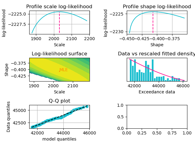
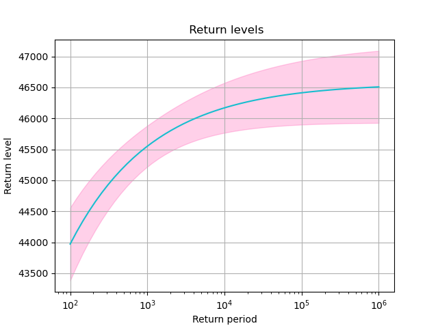
Return levels for GB
Bivariate extreme value modelling
Bivariate EV models are built analogously to univariate models. When fitting a bivarate tail model there is a choice between assuming "strong" or "weak" association between extreme co-occurrences across components 1. The package implements a Bayesian factor test, shown below, to help justify this decision. In addition, marginal distributions can be passed to be used for quantile estimation in the fitting procedure.
Data sample scatterplot (x-axis: GB, y-axis: DK)
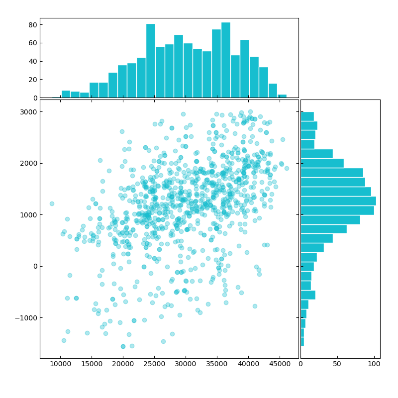
# set random seed
np.random.seed(1)
# instantiate bivariate empirical object with net demand from both areas
bivar_empirical = bivar.Empirical.from_data(np.stack([gb_nd, dk_nd], axis=1))
bivar_empirical.plot();plt.show()
# test for asymptotic dependence and fit corresponding model
r = bivar_empirical.test_asymptotic_dependence(q_th)
if r > 1: # r > 1 suggests strong association between extremes
model = "logistic"
else: # r <= 1 suggests weak association between extremes
model = "gaussian"
bivar_ev_model = bivar_empirical.fit_tail_model(
model = model,
quantile_threshold = q_th,
margin1 = gb_dist_ev,
margin2 = dk_dist_ev)
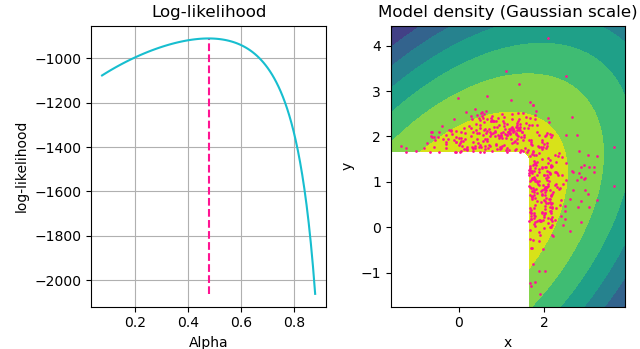
bivar_ev_model.plot_diagnostics();plt.show()
Bivariate model's diagnostics plots
Energy procurement modelling
For the sake of this example, synthetic conventional generator fleets are going to be created for both areas in order to compute risk indices for a hypothetical interconnected system.
from riskmodels.adequacy import acg_models
# get number of timesteps in peak season
n = len(gb_nd)

# assume a base fleet of 200 generators with 240 max. capacity and 4% breakdown rate
uk_gen_df = pd.DataFrame([{"capacity": 240, "availability": 0.96} for k in range(200)])
uk_gen = acg_models.NonSequential.from_generator_df(uk_gen_df)

# assume a base fleet of 55 generators with 61 max. capacity and 4% breakdown rate
dk_gen_df = pd.DataFrame([{"capacity": 61, "availability": 0.96} for k in range(55)])
dk_gen = acg_models.NonSequential.from_generator_df(dk_gen_df)

# define LOLE functon
def lole(gen, net_demand, n=n):
  #Integer distributions can be convolved with other integer or continuous distributions through the + operator
  return n*(1 - (-gen + net_demand).cdf(0))

# compute pre-interconnection LOLEs
lole(dk_gen, dk_dist_ev)

lole(uk_gen, gb_dist_ev)
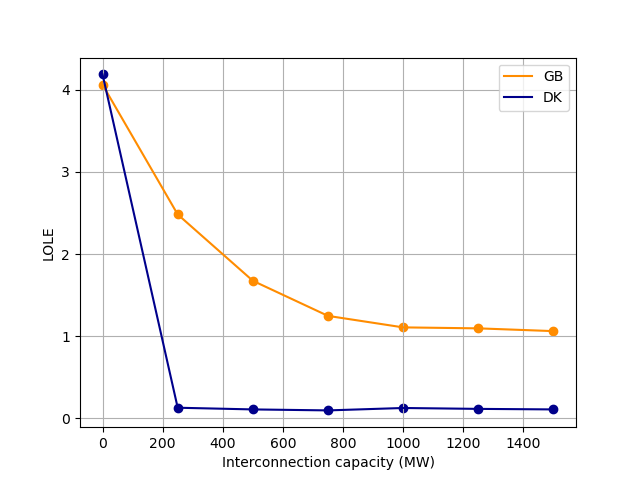
LOLE can be computed exactly for univariate surplus distributions as above, but post-interconnection LOLE requires Monte Carlo estimation. Below, post-interconnection LOLEs are computed for both areas for a range of interconnection capacities up to 1.5 GW.
bivariate_gen = bivar.Independent(x=uk_gen, y=dk_gen)

from riskmodels.adequacy.capacity_models import BivariateNSMonteCarlo

bivariate_surplus = BivariateNSMonteCarlo(
  gen_distribution = bivariate_gen,
  net_demand = bivar_ev_model,
  season_length = n,
  size = 5000000)

itc_caps = np.linspace(0, 1500, 7)

gb_post_itc_lole = np.array([bivariate_surplus.lole(area=0, itc_cap = itc_cap) for itc_cap in itc_caps])
dk_post_itc_lole = np.array([bivariate_surplus.lole(area=1, itc_cap = itc_cap) for itc_cap in itc_caps])

plt.plot(itc_caps, gb_post_itc_lole, color="darkorange", label = "GB")
plt.scatter(itc_caps, gb_post_itc_lole, color="darkorange")

plt.plot(itc_caps, dk_post_itc_lole, color="darkblue", label = "DK")
plt.scatter(itc_caps, dk_post_itc_lole, color="darkblue")

plt.xlabel("Interconnection capacity (MW)")
plt.ylabel("LOLE")
plt.grid()
plt.legend()
plt.show()
Post-interconnection LOLE indices
1: A more in-depth explanation of asymptotic dependence vs independence is given in 'Statistics of Extremes: Theory and Applications' by Beirlant et al, page 342.


Download files
Download the file for your platform. If you're not sure which to choose, learn more about installing packages.
Source Distribution
File details
Details for the file riskmodels-2.3.0.tar.gz.
File metadata
- Download URL: riskmodels-2.3.0.tar.gz
- Upload date:
- Size: 107.3 kB
- Tags: Source
- Uploaded using Trusted Publishing? No
- Uploaded via: twine/4.0.2 CPython/3.9.17
File hashes
| Algorithm | Hash digest | |
|---|---|---|
| SHA256 |
b35f05941da15f08ede1c8cda0fb4afbed970c07783a4ef4146b5a2d7b946bac
|
|
| MD5 |
3d6d6aaf9a669f62fa081c19e55c8b44
|
|
| BLAKE2b-256 |
ac33f07dac1c0e22ef94471eee1fbb0561bd654e4482709146acfe3a0d674680
|


