'Runge-Kutta adaptive-step and constant-step solvers for nonlinear PDEs'

Project description


rkstiff
Exponential time–differencing (ETD) and integrating factor (IF) Runge–Kutta solvers for stiff semi-linear PDEs:
$u_t = L u + \mathrm{NL}(u)$
- Fast, adaptive, and pure Python (NumPy/SciPy only)
- Embedded error control, logging, and flexible operator support
- Designed for spectral methods and diagonalizable systems
Tested: Python 3.9–3.13 | Dependencies: NumPy, SciPy | Optional: matplotlib, jupyter, pytest
Docs: rkstiff.readthedocs.io
Features
- Adaptive ETD/IF Runge–Kutta solvers: ETD35, ETD34, IF34, IF45DP (embedded error control)
- Fixed-step solvers: ETD4, ETD5, IF4
- Operator flexibility: Diagonal or full matrix (spectral/finite-difference)
- Spectral methods: Fourier/Chebyshev support
- Configurable error control:
SolverConfigfor tolerances, safety factors - Logging: Per-solver logging, adjustable verbosity
- Lightweight API: Pass a linear operator array and a callable nonlinear function
- Utility modules: Grids, spectral derivatives, transforms, models, logging helpers
Supported equations: Nonlinear Schrödinger, Kuramoto–Sivashinsky, Korteweg–de Vries, Burgers, Allen–Cahn, Sine–Gordon
Installation
pip (recommended):
python -m pip install rkstiff
conda-forge:
conda create -n rkstiff-env -c conda-forge rkstiff
conda activate rkstiff-env
From source:
git clone https://github.com/whalenpt/rkstiff.git
cd rkstiff
python -m pip install .
Extras:
# demos: matplotlib + jupyter; tests: pytest
python -m pip install "rkstiff[demo]"
python -m pip install "rkstiff[test]"
Quickstart Example (Kuramoto–Sivashinsky)
import numpy as np
from rkstiff import grids, if34

# Real-valued grid for rfft
n = 1024
a, b = 0.0, 32.0 * np.pi
x, kx = grids.construct_x_kx_rfft(n, a, b)

# Linear operator in Fourier space
lin_op = kx**2 * (1 - kx**2)

# Nonlinear term: -F{ u * u_x }
def nl_func(u_fft):
    u = np.fft.irfft(u_fft)
    ux = np.fft.irfft(1j * kx * u_fft)
    return -np.fft.rfft(u * ux)

# Initial condition in real space → Fourier space
u0 = np.cos(x / 16) * (1.0 + np.sin(x / 16))
u0_fft = np.fft.rfft(u0)

solver = if34.IF34(lin_op=lin_op, nl_func=nl_func)
uf_fft = solver.evolve(u0_fft, t0=0.0, tf=50.0, store_freq=20)

# Convert stored Fourier snapshots back to real space
U = np.array([np.fft.irfft(s) for s in solver.u])  # shape: (num_snaps, n)
t = np.array(solver.t)
solver.uandsolver.tstore snapshots everystore_freqinternal steps;evolvereturns the final state.
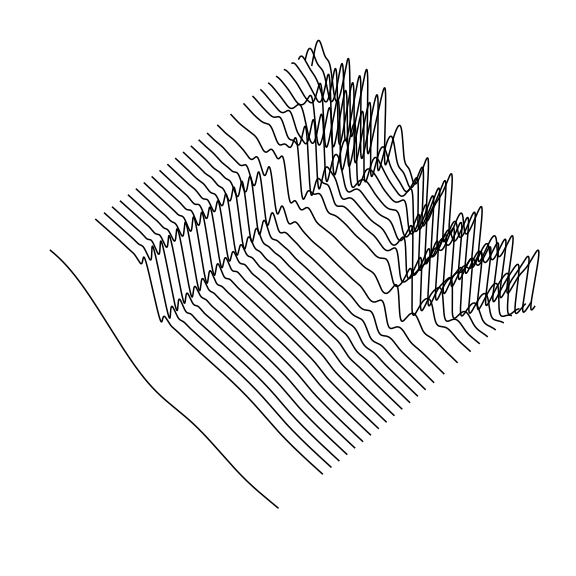
Kuramoto–Sivashinsky chaotic field propagation using IF34.
💡 More examples:
Several fully runnable Jupyter notebooks are included in thedemos/folder.
Each notebook illustrates solver usage, adaptive-step control, and visualization for different PDEs
(e.g., Kuramoto–Sivashinsky, NLS, and Allen–Cahn).
To try them:python -m pip install "rkstiff[demo]" jupyter notebook demos/
API Overview
Solver Classes
| Solver | Module | Order (embedded) | Adaptive | Notes |
|---|---|---|---|---|
ETD35 |
etd35 |
5 (3) | ✅ | Best for diagonalized systems |
ETD34 |
etd34 |
4 (3) | ✅ | Krogstad 4th order |
IF34 |
if34 |
4 (3) | ✅ | Integrating factor |
IF45DP |
if45dp |
5 (4) | ✅ | Dormand–Prince IF |
ETD4 |
etd4 |
4 (–) | ❌ | Krogstad fixed-step |
ETD5 |
etd5 |
5 (–) | ❌ | Same base as ETD35 |
IF4 |
if4 |
4 (–) | ❌ | Fixed-step IF |
Constructor Signature (Adaptive Classes)
Solver(lin_op: np.ndarray, nl_func: Callable[[np.ndarray], np.ndarray], config: SolverConfig = ..., loglevel: str = ...)
lin_op: array shaped likeu, typically diagonal entries in the working basisnl_func(u): returns nonlinear term in same basisconfig: error control and adaptivity (optional; defaults to SolverConfig())loglevel: logging verbosity (optional; defaults to "INFO")
Configuration & Logging
Adaptive Error Control
Configure embedded error estimation and adaptive step control via SolverConfig:
from rkstiff.if34 import IF34
from rkstiff.solveras import SolverConfig

config = SolverConfig(epsilon=1e-5, incr_f=1.2, decr_f=0.8, safety_f=0.9)
solver = IF34(lin_op, nl_func, config=config, loglevel="INFO")
Parameter notes (typical meanings):
epsilon: target local error tolerance for the embedded pair.safety_f: safety factor applied to proposed step-size updates.incr_f/decr_f: bounds on how muchdtmay grow/shrink on accept/reject.- (Implementation-specific fields may exist; see docs for full list and defaults.)
Logging
Set logging level per solver:
solver = IF34(lin_op, nl_func, loglevel="DEBUG")
Utility Modules
grids: Grid and wavenumber construction for FFT/RFFT/Chebyshevderivatives: Spectral differentiation (FFT, RFFT, Chebyshev)transforms: Basis transformsmodels: Example PDEsutil.loghelper: Logging setup and control
Usage Tips
- For spectral methods, pass
lin_opin Fourier space and implementnl_funcin that same space - For diagonalizable systems, pre-diagonalize once and reuse that basis
- ETD methods may precompute φ-functions; reuse the solver instance for speed
- Storage:
solver.uandsolver.thold snapshots; control frequency withstore_freq
Testing & Coverage
Run tests and view coverage:
python -m pip install "rkstiff[test]"
pytest
Citation
If you use rkstiff in academic work, please cite:
P. Whalen, M. Brio, J.V. Moloney, Exponential time-differencing with embedded Runge–Kutta adaptive step control, Journal of Computational Physics 280 (2015) 579–601. DOI: 10.1016/j.jcp.2014.09.038
@article{WhalenBrioMoloney2015,
  title   = {Exponential time-differencing with embedded Runge--Kutta adaptive step control},
  author  = {Whalen, P. and Brio, M. and Moloney, J. V.},
  journal = {Journal of Computational Physics},
  volume  = {280},
  pages   = {579--601},
  year    = {2015},
  doi     = {10.1016/j.jcp.2014.09.038}
}
License
MIT — see LICENSE for details.
Contact
Patrick Whalen — whalenpt@gmail.com
Release history Release notifications | RSS feed


Download files
Download the file for your platform. If you're not sure which to choose, learn more about installing packages.
Source Distribution
Built Distribution
Filter files by name, interpreter, ABI, and platform.
If you're not sure about the file name format, learn more about wheel file names.
Copy a direct link to the current filters
File details
Details for the file rkstiff-1.0.0.tar.gz.
File metadata
- Download URL: rkstiff-1.0.0.tar.gz
- Upload date:
- Size: 204.6 kB
- Tags: Source
- Uploaded using Trusted Publishing? No
- Uploaded via: twine/6.2.0 CPython/3.9.25
File hashes
| Algorithm | Hash digest | |
|---|---|---|
| SHA256 |
5be4c30913339041b922feb35595ff1c400950f92bcb2f43e836d49a7a87a57b
|
|
| MD5 |
3ea091d38542fe50b61dbc109ceac015
|
|
| BLAKE2b-256 |
fe43d57a3e9b478d8cd214cf245b3df843a5d89c62426819ad2bbc0ce528e6ef
|
File details
Details for the file rkstiff-1.0.0-py3-none-any.whl.
File metadata
- Download URL: rkstiff-1.0.0-py3-none-any.whl
- Upload date:
- Size: 63.2 kB
- Tags: Python 3
- Uploaded using Trusted Publishing? No
- Uploaded via: twine/6.2.0 CPython/3.9.25
File hashes
| Algorithm | Hash digest | |
|---|---|---|
| SHA256 |
ffaadfda3165dbb143a7c2ef58acc5108e20a553309af0ae4a7c8702cc184024
|
|
| MD5 |
ec11c176892fffff25f6f06bdd6c8ce0
|
|
| BLAKE2b-256 |
82ecf9dda97d28854c16ef732a2479c3e0af07db2317dcccb54c27021183fabc
|


