Probabilistic Methods of Parameter Inference for ODEs

Project description
rodeo: Probabilistic Methods of Parameter Inference for Ordinary Differential Equations
Home | Installation | Documentation | Tutorial | Developers | Change logs

Description
rodeo is a fast Python library that uses probabilistic numerics to solve ordinary differential equations (ODEs). That is, most ODE solvers (such as Euler's method) produce a deterministic approximation to the ODE on a grid of step size $\Delta t$. As $\Delta t$ goes to zero, the approximation converges to the true ODE solution. Probabilistic solvers also output a solution on a grid of size $\Delta t$; however, the solution is random. Still, as $\Delta t$ goes to zero, the probabilistic numerical approximation converges to the true solution.
rodeo provides a lightweight and extensible family of approximations to a nonlinear Bayesian filtering paradigm common to many probabilistic solvers (Tronarp et al (2018)). This begins by putting a Gaussian process prior on the ODE solution, and updating it sequentially as the solver steps through the grid. rodeo is built on jax which allows for just-in-time compilation and auto-differentiation. The API of jax is almost equivalent to that of numpy.
rodeo provides two main tools: one for approximating the ODE solution and the other for parameter inference. For the former we provide:
solve: Implementation of a probabilistic ODE solver which uses a nonlinear Bayesian filtering paradigm.
For the latter we provide the likelihood approximation methods:
basic: Implementation of a basic likelihood approximation method (details can be found in Wu and Lysy (2024)).fenrir: Implementation of Fenrir (Tronarp et al (2022)).dalton: Implementation of the data-adaptive ODE likelihood approximation (Wu and Lysy (2024)).pseudo_marginal: Implementation of Chkrebtii's marginal MCMC algorithm (Chkrebtii et al (2016)).magi: Implementation of MAGI (Wong et al (2023)) with a Markov prior.
Detailed examples for their usage can be found in the Documentation section. Please note that this is the jax-only version of rodeo. For the legacy versions using various other backends please see here.
Installation
Download the repo from GitHub and then install with the setup.cfg script:
git clone https://github.com/mlysy/rodeo.git
cd rodeo
pip install .
Documentation
Please first go to readthedocs to see the rendered documentation for the following examples.
-
A quickstart tutorial on solving a simple ODE problem.
-
An example for solving a higher-ordered ODE.
-
An example for solving a difficult chaotic ODE.
-
An example of a parameter inference problem where we use the Laplace approximation.
Walkthrough
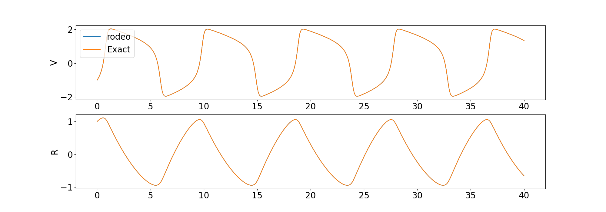
In this walkthrough, we show both how to solve an ODE with our probabilistic solver and conduct parameter inference. We will first illustrate the set-up for solving the ODE. To that end, let's consider the following first ordered ODE example (FitzHugh-Nagumo model),
$$ \begin{align*} \frac{dV}{dt} &= c(V - \frac{V^3}{3} + R), \ \frac{dR}{dt} &= -\frac{(V - a + bR)}{c}, \ X(t) &= (V(0), R(0)) = (-1,1). \end{align*} $$
where the solution $X(t)$ is sought on the interval $t \in [0, 40]$ and $\theta = (a,b,c) = (.2,.2,3)$.
Following the notation of Wu and Lysy (2024), we have $p-1=1$ in this example. To approximate the solution with the probabilistic solver, we use a simple Gaussian process prior proposed by Schober et al (2019); namely, that $V(t)$ and $R(t)$ are independent $q-1$ times integrated Brownian motion, such that
$$ \begin{equation*} x^{(q)}(t) = \sigma_x B(t) \end{equation*} $$
for $x=V, R$. The result is a $q$-dimensional continuous Gaussian Markov process $\boldsymbol{x(t)} = \big(x^{(0)}(t), x^{(1)}(t), \ldots, x^{(q-1)}(t)\big)$ for each variable $x=V, R$. Here $x^{(i)}(t)$ denotes the $i$-th derivative of $x(t)$. The IBM model specifies that each of these is continuous, but $x^{(q)}(t)$ is not. Therefore, we need to pick $q \geq p$. It's usually a good idea to have $q$ a bit larger than $p$, especially when we think that the true solution $X(t)$ is smooth. However, increasing $q$ also increases the computational burden, and doesn't necessarily have to be large for the solver to work. For this example, we will use $q=3$. To initialize, we simply set $\boldsymbol{X(0)} = (V^{(0)}(0), V^{(1)}(0), 0, R^{(0)}(0), R^{(1)}(0), 0)$ where we padded the initial value with zeros for the higher derivative. The Python code to implement all this is as follows.
import jax
import jax.numpy as jnp
import rodeo

def fitz_fun(X, t, **params):
    "FitzHugh-Nagumo ODE in rodeo format."
    a, b, c = params["theta"]
    V, R = X[:, 0]
    return jnp.array(
        [[c * (V - V * V * V / 3 + R)],
         [-1 / c * (V - a + b * R)]]
    )

n_vars = 2  # number of variables in the ODE
n_deriv = 3  # max number of derivatives

x0 = jnp.array([-1., 1.])  # initial value for the ODE-IVP
theta = jnp.array([.2, .2, 3])  # ODE parameters

# we have a helper function to help with the rodeo initialization
W, fitz_init_pad = rodeo.utils.first_order_pad(fitz_fun, n_vars, n_deriv)
# fitz_init_pad takes Args:
# x0: initial value for the ODE-ivp
# t: initial time
# **params: extra model parameters as kwargs
X0 = fitz_init_pad(x0, 0., theta=theta)  # initial value in rodeo format

# Time interval on which a solution is sought.
t_min = 0.
t_max = 40.

# --- Define the prior process -------------------------------------------

sigma = jnp.array([.1] * n_vars)  # IBM process scale factor


# --- data simulation ------------------------------------------------------

n_steps = 800  # number of evaluations steps
dt = (t_max - t_min) / n_steps  # step size

# generate the Kalman parameters corresponding to the prior
prior_pars = rodeo.prior.ibm_init(
    dt=dt,
    n_deriv=n_deriv,
    sigma=sigma
)

# Produce a Pseudo-RNG key
key = jax.random.PRNGKey(0)

Xt, _ = rodeo.solve_mv(
    key=key,
    # define ode
    ode_fun=fitz_fun,
    ode_weight=W,
    ode_init=X0,
    t_min=t_min,
    t_max=t_max,
    theta=theta,  # ODE parameters added here
    # solver parameters
    n_steps=n_steps,
    interrogate=rodeo.interrogate.interrogate_kramer,
    prior_pars=prior_pars
)
We compare the solution from the solver to the deterministic solution provided by odeint in the scipy library.
We also include examples for solving a higher-ordered ODE and a chaotic ODE.
Parameter Inference
We now move to the parameter inference problem. rodeo contains several likelihood approximation methods summarized in the Description section.
Here, we will use the basic likelihood approximation method. Suppose observations are simulated via the model
$$ Y(t) \sim \textnormal{Normal}(X(t), \phi^2 \cdot \boldsymbol{I}_{2\times 2}) $$
where $t=0, 1, \ldots, 40$ and $\phi^2 = 0.005$. The parameters of interest are $\boldsymbol{\Theta} = (a, b, c, V(0), R(0))$ with $a,b,c > 0$.
We use a normal prior for $(\log a, \log b, \log c, V(0), R(0))$ with mean $0$ and standard deivation $10$.
The following function can be used to construct the basic likelihood approximation for $\boldsymbol{\Theta}$.
def fitz_logprior(upars):
    "Logprior on unconstrained model parameters."
    n_theta = 5  # number of ODE + IV parameters
    lpi = jax.scipy.stats.norm.logpdf(
        x=upars[:n_theta],
        loc=0.,
        scale=10.
    )
    return jnp.sum(lpi)


def fitz_loglik(obs_data, ode_data, **params):
    """
    Loglikelihood for measurement model.

    Args:
        obs_data (ndarray(n_obs, n_vars)): Observations data.
        ode_data (ndarray(n_obs, n_vars, n_deriv)): ODE solution.
    """
    ll = jax.scipy.stats.norm.logpdf(
        x=obs_data,
        loc=ode_data[:, :, 0],
        scale=0.005
    )
    return jnp.sum(ll)


def constrain_pars(upars, dt):
    """
    Convert unconstrained optimization parameters into rodeo inputs.

    Args:
        upars : Parameters vector on unconstrainted scale.
        dt : Discretization grid size.

    Returns:
        tuple with elements:
        - theta : ODE parameters.
        - X0 : Initial values in rodeo format.
        - prior_pars : Prior matrices.
    """
    theta = jnp.exp(upars[:3])
    x0 = upars[3:5]
    X0 = fitz_init_pad(x0, 0, theta=theta)
    sigma = upars[5:]
    prior_pars = rodeo.prior.ibm_init(
        dt=dt,
        n_deriv=n_deriv,
        sigma=sigma
    )
    return theta, X0, prior_pars


def neglogpost_basic(upars):
    "Negative logposterior for basic approximation."
    # solve ODE
    theta, X0, prior_pars = constrain_pars(upars, dt)
    # basic loglikelihood
    ll = rodeo.inference.basic(
        key=key,
        # ode specification
        ode_fun=fitz_fun,
        ode_weight=W,
        ode_init=X0,
        t_min=t_min,
        t_max=t_max,
        theta=theta,
        # solver parameters
        n_steps=n_steps,
        interrogate=rodeo.interrogate.interrogate_kramer,
        prior_pars=prior_pars,
        # observations
        obs_data=obs_data,
        obs_times=obs_times,
        obs_loglik=fitz_loglik
    )
    return -(ll + fitz_logprior(upars))
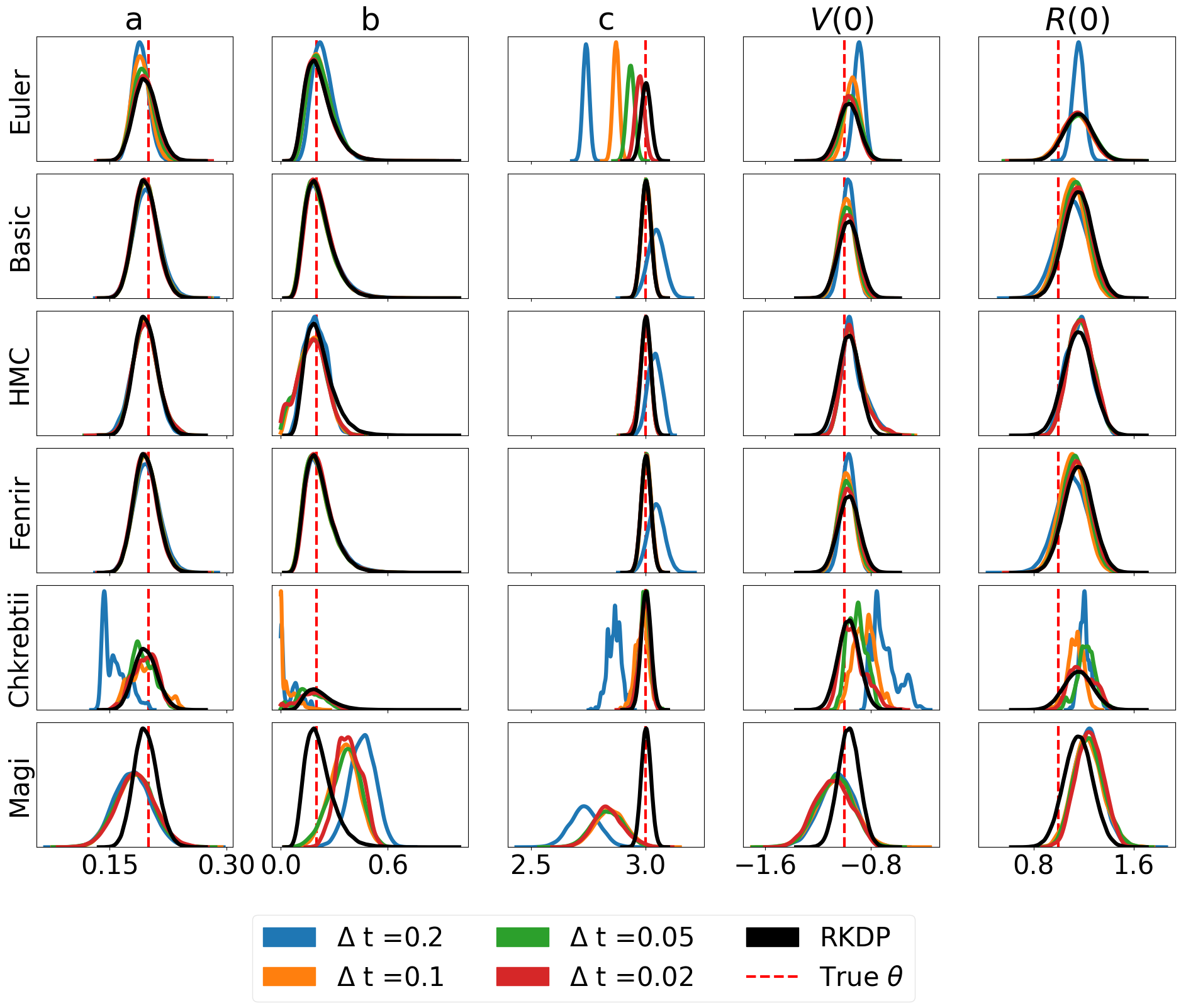
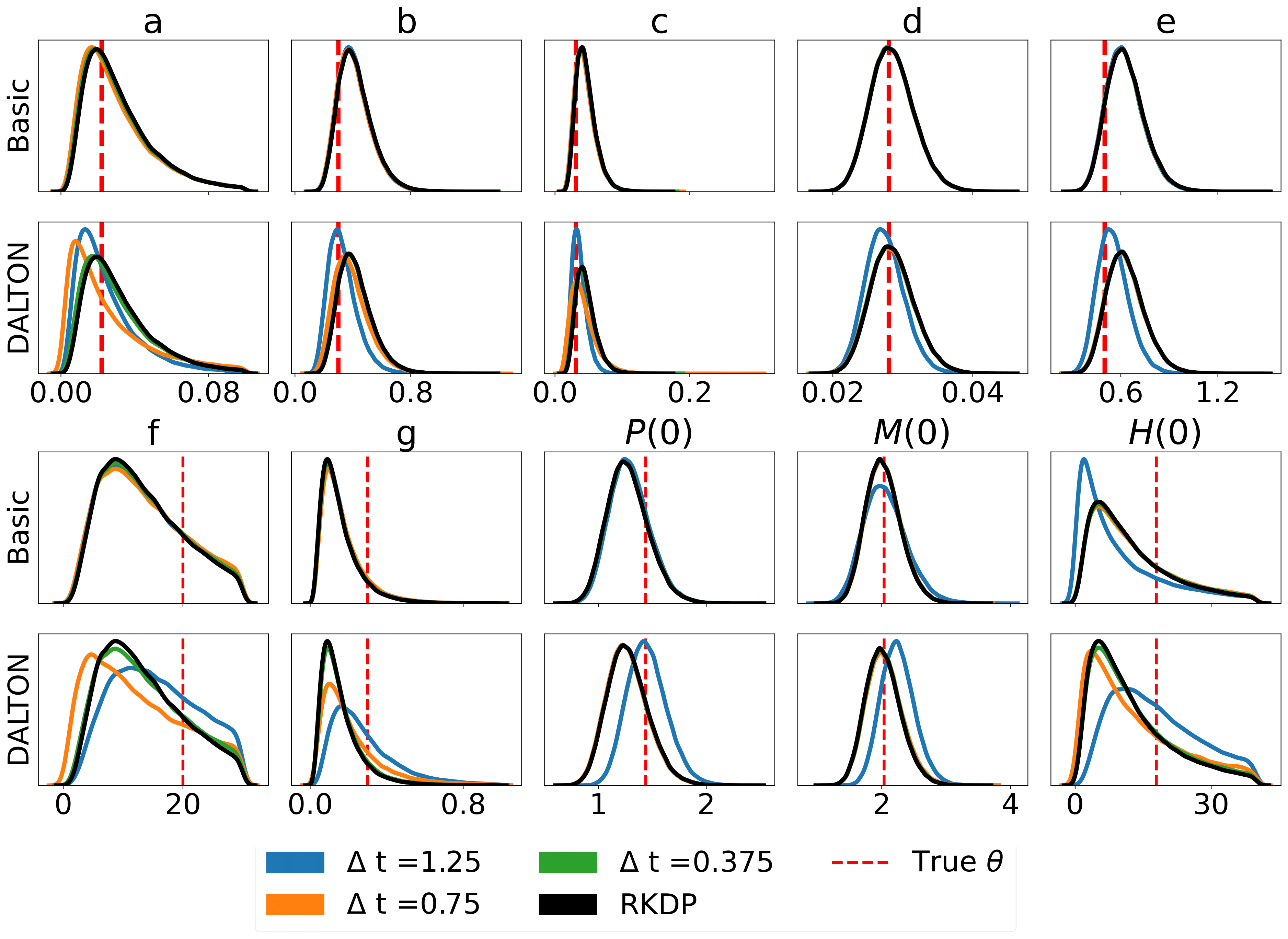
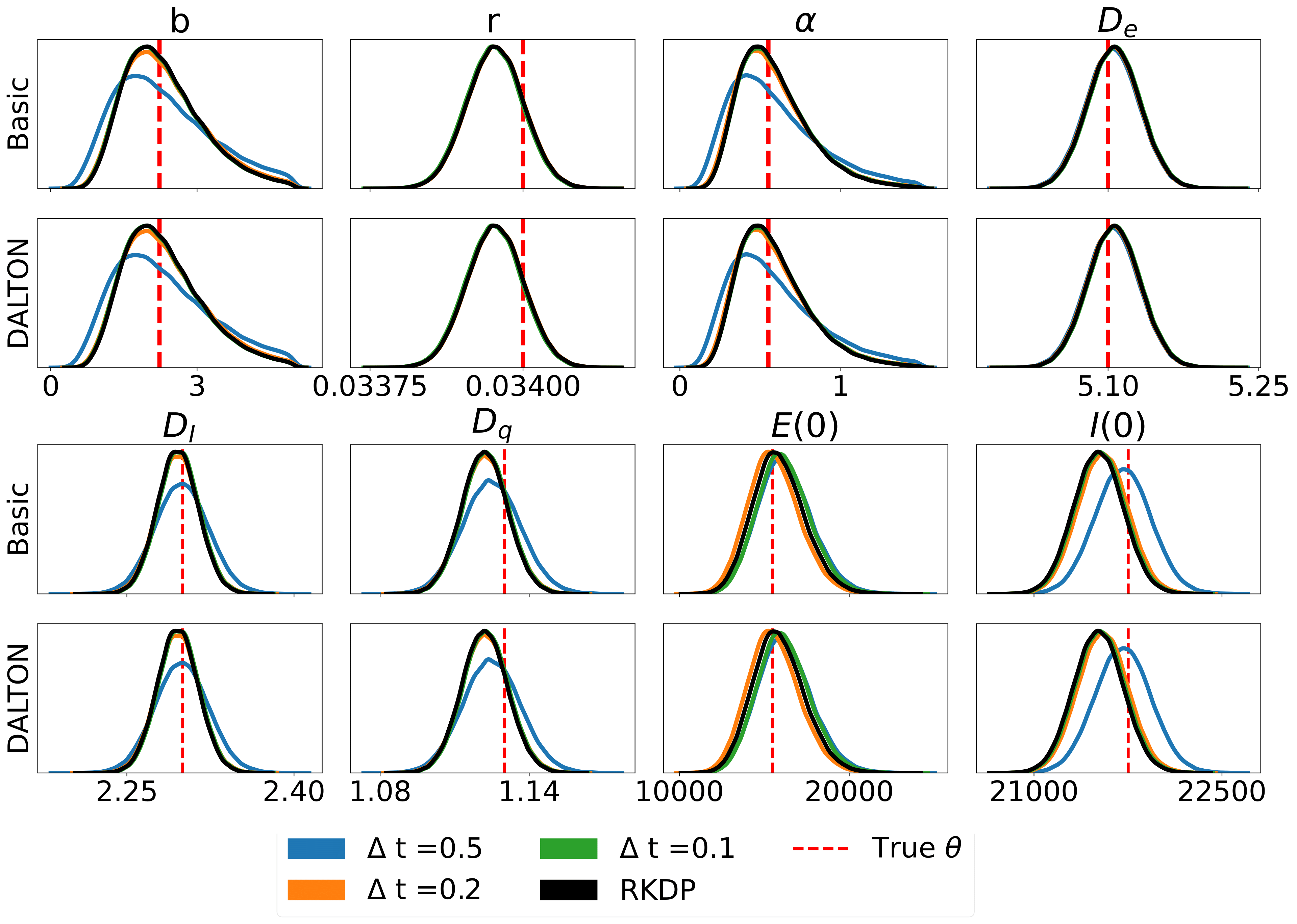
This is a basic example to demonstrate usage. We suggest more sophisticated likelihood approximations which propagate the solution uncertainty to the likelihood approximation such as fenrir, marginal_mcmc and dalton. Please refer to the parameter inference tutorial for more details.
Results
Here are some results produced by various likelihood approximations found in rodeo from /examples/:
FitzHugh-Nagumo
Hes1
SEIRAH
Developers
Unit Testing
The unit tests can be ran through the following commands:
cd tests
python -m unittest discover -v
Or, install tox, then from within rodeo enter command line: tox.
Building Documentation
The HTML documentation can be compiled from the root folder:
pip install .[docs]
cd docs
make html
This will create the documentation in docs/build.


Download files
Download the file for your platform. If you're not sure which to choose, learn more about installing packages.
Source Distribution
Built Distribution
Filter files by name, interpreter, ABI, and platform.
If you're not sure about the file name format, learn more about wheel file names.
Copy a direct link to the current filters
File details
Details for the file rodeo-1.1.3.tar.gz.
File metadata
- Download URL: rodeo-1.1.3.tar.gz
- Upload date:
- Size: 38.0 kB
- Tags: Source
- Uploaded using Trusted Publishing? No
- Uploaded via: twine/6.1.0 CPython/3.9.19
File hashes
| Algorithm | Hash digest | |
|---|---|---|
| SHA256 |
aaf4be029b8102f66444a94f334e1ae12c573018fb1f89bb8f9435eb825aef44
|
|
| MD5 |
e12b1604dd8549d901b977c9fc8da0c1
|
|
| BLAKE2b-256 |
36ee61a404128a23c242ff53b5338e8ab47b0f859527f841cabc2ede940748b7
|
File details
Details for the file rodeo-1.1.3-py3-none-any.whl.
File metadata
- Download URL: rodeo-1.1.3-py3-none-any.whl
- Upload date:
- Size: 37.9 kB
- Tags: Python 3
- Uploaded using Trusted Publishing? No
- Uploaded via: twine/6.1.0 CPython/3.9.19
File hashes
| Algorithm | Hash digest | |
|---|---|---|
| SHA256 |
e3aaa105953a55936ee8165c9777c4c012dfefdf56d86e6001c91b0388be8afb
|
|
| MD5 |
682d6a8f31a4a0b8b0a2206195586249
|
|
| BLAKE2b-256 |
d0ec73649ffe83167fd74503abe82f80e7ee738945691ff99b4a288ea1780987
|


