No project description provided

Project description

This file is also available as README.nb Mathematica notebook that replicates all derivations and plots.
s-curve-beta: Efficient Python implementation of the smoothest S-curve robot motion planner ever
- It's 2022 and you're still using a trapezoid motion profile?
- Your robot is vibrating like a vacuum machine?
- Tired of the mess in the code because of the multiple piecewise time regions?
- Want a simple single-formula smooth motion profile?
- Want an S-curve implementation that literally fits in 20 lines of code?
If you answer "yes" to any of the above, read on.
Based on the answer of Cuye Waldman (https://math.stackexchange.com/a/2403818) I present this Python package to calculate the S-curve for the robot motion planning with a given maximum velocity and acceleration with a single formula.
Here is the complete motion formula:
$$f\left( t, p \right)=\frac{1}{2}\left[ 1+\text{sgn} (x),\frac{B\left( {1}/{2};,p+1,{t^2} \right)}{B\left( {1}/{2};,p+1 \right)} \right],$$
$$motionTime(robotVmax, robotAmax,motionRange)=\ max\left[\frac{23^{3/4}}{\sqrt{\pi}}\sqrt\frac{motionRange}{robotAmax},\frac{32}{5\pi}*\frac{motionRange}{robotVmax}\right],$$
$$position(t,robotVmax,robotAmax,motionRange)=\ motionRange*f\left(\frac{2 t}{motionTime}-1,2.5\right),$$
where sgn(x) is Sign function, numerator and denominator 𝐵s are the incomplete and complete beta functions, respectively (that's where beta comes from in the name), robotAmax is the maximum acceleration and motionRange is the absolute value of the motion (from start to end).
Here are 2 examples of motion planning with $motionRange=2$:

The motion curve always has the same shape, while horizontal and vertical scales change. This property has the following benefits:
- The maximum jerk is smaller compared to the case where you accelerate to the maximum velocity, stay there for a while and then decelerate.
- The curve (function $f(t,2.5)$ for $-1\le t \le 1$) can be precomputed, so instead of calculating Beta functions each time it's possible to do the linear interpolation of the precomputed points.
Installation
Using pip (recommended):
pip install s-curve-beta
From source:
git clone https://github.com/hidoba/s-curve-beta.git
cd s-curve-beta
python setup.py install
Examples
Calculating robot position at given moments of time:
import scurvebeta as scb

# motion parameters
max_velocity = 12
max_acceleration = 3
x0 = -3
x1 = 10

# Calculate motion time
motionTime = scb.motionTime(max_velocity, max_acceleration, abs(x0-x1))
print("motionTime = ", motionTime, "seconds")

# Calculate position at a given time
t = 2.3
print("position(",t,") = ", scb.sCurve(t, motionTime, x0, x1))

# Calculate multiple positions at given moments of time (faster, most recommended)
import numpy as np
t = np.array([-1,0,1,2,3,motionTime,10])
print("position(",t,") = ", scb.sCurve(t, motionTime, x0, x1))
Making plots:
import scurvebeta as scb
import matplotlib.pyplot as plt
import numpy as np
def plotMotion(max_velocity, max_acceleration, x0, x1):
motionTime = scb.motionTime(max_velocity, max_acceleration, abs(x0-x1))
dt = 0.08
t = np.arange(0,motionTime, dt)
pos = scb.sCurve(t, motionTime, x0, x1)
vel = np.diff(pos)/dt
acc = np.diff(vel)/dt
jerk = np.diff(acc)/dt
fig, axs = plt.subplots(2, 1)
axs[0].plot(t, pos)
axs[0].set_ylabel('Position')
axs[0].grid(True)
axs[1].plot(t[:-1], vel, label='velocity')
axs[1].plot(t[:-2], acc, label='acceleration')
axs[1].plot(t[:-3], jerk, label='jerk')
axs[1].axhline(y = max_acceleration, color = 'orange', linestyle = '--')
axs[1].axhline(y = max_velocity, color = 'blue', linestyle = '--')
axs[1].text(0,max_acceleration+0.15,'max_acceleration='+str(max_acceleration))
axs[1].text(0,max_velocity+0.15,'max_velocity='+str(max_velocity))
axs[1].grid(True)
axs[1].set_xlabel('Time')
axs[1].legend(handlelength=4)
fig.tight_layout()
plt.show()
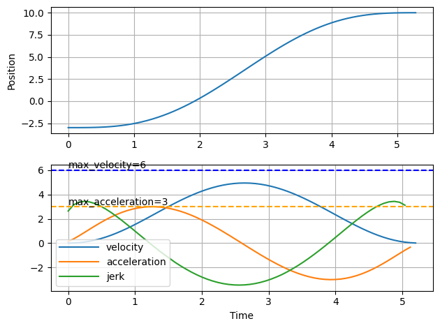
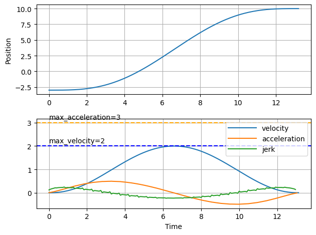
# Please note that if you need more accurate velocity / acceleration
# you should better use the 'true' version of function instead of the 'interpolated' one.
# Pay attention at the jerk on the second plot, the sawteeth are because of imprecision
# of very small changes of the third derivative. If you just need the position,
# interpolated function should be just fine.
plotMotion(6, 3, -3, 10)
plotMotion(2, 3, -3, 10)
Interpolated vs True function
By default s-curve-beta uses an interpolated version of the f function (using 801 points interpolation). It's very fast if used on the arrays and it can be easily adapted for microcontrollers.
You can use the true function (requires scipy) by importing an optional scurvebetatrue module:
from scurvebeta import scurvebetatrue
print(scurvebetatrue.sCurve_true(2.3,15,-1,5))

import scurvebeta as scb
print(scurvebeta.sCurve(2.3,15,-1,5))
-0.8849490453964555
-0.8849435436031998
Compare the execution speed:
import timeit
from scurvebeta import scurvebetatrue
import scurvebeta as scb
import numpy as np

def trueFunction():
    return scurvebetatrue.sCurve_true(2.3,15,-1,5)

def trueFunctionArray():
    return scurvebetatrue.sCurve_true(np.arange(0,15,15/100000),15,-1,5)

def interpolatedFunction():
    return scb.sCurve(2.3,15,-1,5)

def interpolatedFunctionArray():
    return scb.sCurve(np.arange(0,15,15/100000),15,-1,5)

print(timeit.timeit('trueFunction()',number=100000, setup="from __main__ import trueFunction"))
# 0.4408080680000239

timeit.timeit('trueFunctionArray()',number=1, setup="from __main__ import trueFunctionArray")
# 0.4047970910000913

timeit.timeit('interpolatedFunction()',number=100000, setup="from __main__ import interpolatedFunction")
# 0.381616509999958

timeit.timeit('interpolatedFunctionArray()',number=1, setup="from __main__ import interpolatedFunctionArray")
# 0.0019440340000755896
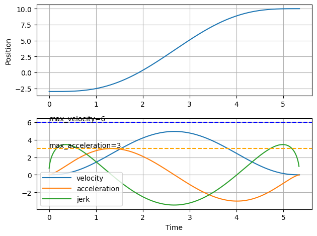
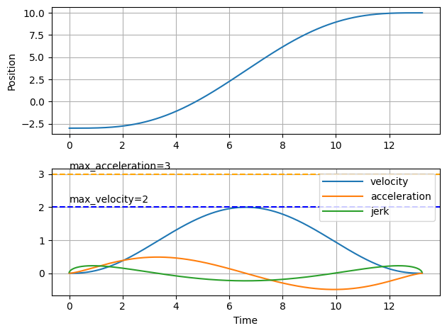
Plots with "True" function:
import scurvebeta as scb
from scurvebeta import scurvebetatrue
import matplotlib.pyplot as plt
import numpy as np

def plotMotionTrue(max_velocity, max_acceleration, x0, x1):
    motionTime = scb.motionTime(max_velocity, max_acceleration, abs(x0-x1))
    dt = 0.005
    t = np.arange(0,motionTime, dt)
    pos = scurvebetatrue.sCurve_true(t, motionTime, x0, x1)
    vel = np.diff(pos)/dt
    acc = np.diff(vel)/dt
    jerk = np.diff(acc)/dt

    fig, axs = plt.subplots(2, 1)
    axs[0].plot(t, pos)
    axs[0].set_ylabel('Position')
    axs[0].grid(True)

    axs[1].plot(t[:-1], vel, label='velocity')
    axs[1].plot(t[:-2], acc, label='acceleration')
    axs[1].plot(t[:-3], jerk, label='jerk')
    axs[1].axhline(y = max_acceleration, color = 'orange', linestyle = '--')
    axs[1].axhline(y = max_velocity, color = 'blue', linestyle = '--')
    axs[1].text(0,max_acceleration+0.15,'max_acceleration='+str(max_acceleration))
    axs[1].text(0,max_velocity+0.15,'max_velocity='+str(max_velocity))
    axs[1].grid(True)
    axs[1].set_xlabel('Time')
    axs[1].legend(handlelength=4)

    fig.tight_layout()
    plt.show()

plotMotionTrue(6, 3, -3, 10)
plotMotionTrue(2, 3, -3, 10)
Multiple axes synchronization
To synchronize multiple axes simply calculate the maximum motion time of all axes and use it for every axis. This will minimize the maximum jerk and acceleration of the initially faster axes, decreasing the vibrations of the robot.
Derivations
Below derivations include Mathematica code that can be used to replicate them.
This file is also available as README.nb Mathematica notebook that replicates all derivations and plots.
The original f function comes from the integration of the superparabola, done by Cuye Waldman. We can prove that his integration is correct:
f[x_, p_] :=
 1/2 (1 + RealSign[x]*Beta[x^2, 1/2, p + 1]/Beta[1/2, p + 1])

FullSimplify[
 Integrate[(1 - x^2)^p/Beta[1/2, 1 + p], {x, -1, t}] - f[t, p],
 Element[p, Reals] && Element[t, Reals] && 0 <= t < 1 && p > -1]

 (* 0 *)
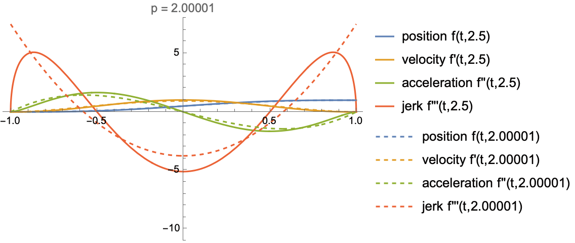
Proof that the most optimal $p$ is 2.5
My suggested value of $p$ is 2.5 which gives the lowest possible absolute jerk, let's see why.
Visualizing derivatives with different values of $p$:
Animate[
 Show[
  Plot[Evaluate@Table[D[f[x, 2.5], {x, i}], {i, 0, 3}], {x, -1, 1},
   PlotLegends -> {"position f(t,2.5)", "velocity f'(t,2.5)",
     "acceleration f''(t,2.5)", "jerk f'''(t,2.5)"},
   PlotRange -> {-11, 8}, PlotLabel -> "p = " ~~ ToString[param]],
  Plot[Evaluate@Table[D[f[x, param], {x, i}], {i, 0, 3}], {x, -1, 1},
   PlotLegends -> (StringJoin[#,
        "(t," ~~ ToString[param] ~~ ")"] & /@ {"position f",
       "velocity f'", "acceleration f''", "jerk f'''"}),
   PlotRange -> All, PlotStyle -> Dashed]
  ],
 {param, 2.00001, 5, 0.15}]
Calculating largest jerks for different values of the parameter $p$:
jerkValues[param_] := {Limit[D[f[x, param], {x, 3}], x -> 0],
  Maximize[{D[f[x, param], {x, 3}], -1 <= x <= 1}, x][[1]]}}

paramData = Table[{p, jerkValues[p]}, {p, 2.001, 3, 0.01}];

ListLinePlot[
 Abs[Transpose[(Outer[List, {#1}, #2][[1]] & @@@ paramData)]],
 PlotLegends -> {"|max negative jerk| (at x=0)", "max positive jerk"},
  Epilog -> {Dashed, InfiniteLine[{2.5, 0}, {0, 1}]},
 AxesLabel -> {"p", "max jerk"}]
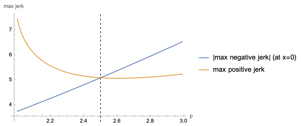
The best value of the parameter $p$ happens to be 2.5, where the max absolute jerk is the smallest.
Discussion on $2\le p<2.5$
It's possible to achieve slightly lower maximum robot accelerations at $2\le p<2.5$:
param = 2;
Show[
  Plot[Evaluate@Table[D[f[x, 2.5], {x, i}], {i, 0, 3}], {x, -1, 1}, PlotLegends -> {"position f(t,2.5)", "velocity f'(t,2.5)", "acceleration f''(t,2.5)", "jerk f'''(t,2.5)"}, PlotRange -> All],
  Plot[Evaluate@Table[D[f[x, param], {x, i}], {i, 0, 3}], {x, -1, 1}, PlotLegends -> (StringJoin[#, "(t," ~~ ToString[param] ~~ ")"] & /@ {"position f", "velocity f'", "acceleration f''", "jerk f'''"}), PlotRange -> All, PlotStyle -> Dashed]
 ]
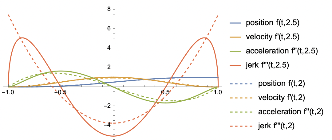
Values of $2\le p<2.5$ can shorten the robot motion time a little bit at the cost of increased maximum jerk hence increased robot vibrations at the beginning and at the end of the motion. I have decided not to implement this at the moment.
Rescaling function f for the particular motion parameters
1. Motion time from the maximum velocity constraint
Max velocity at $t=0$:
maxVelocity = Limit[D[f[x, 5/2], x], x -> 0]
$$\frac{16}{5 \pi}$$
With the given maximum robot velocity robotVmax the shortest motion time can be derived from the equation:
$$robotVmax=\frac{2\frac{16}{5\pi}motionRange}{time}$$
Hence,
$$time = \frac{32}{5 \pi}*\frac{motionRange}{robotVmax}$$
2. Motion time from the maximum acceleration constraint
Calculate max acceleration at $p=2.5$:
FindMaximum[{D[f[x, 5/2], {x, 2}], -1 < x < 0}, x]

(*{1.65399, {x -> -0.5}}*)
Maximum acceleration happens to be at $t=-\frac{1}{2}$
D[f[x, 5/2], {x, 2}] /. x -> -1/2
$$\frac{3\sqrt3}{\pi}$$
With the given maximum robot acceleration robotAmax the shortest motion time can be derived from the equation:
$$\text{robotAmax}=\frac{4\frac{3\sqrt{3}}{\pi }\text{motionRange}}{time^2}$$
Hence,
$$time=\frac{23^{3/4}}{\sqrt{\pi}}\sqrt\frac{motionRange}{robotAmax}$$
3. Motion time with both constraints
To consider both maximum velocity and maximum acceleration constraints we have to take the maximum of the above motion times:
$$motionTime= max\left[\frac{23^{3/4}}{\sqrt{\pi}}\sqrt\frac{motionRange}{robotAmax},\frac{32}{5\pi}*\frac{motionRange}{robotVmax}\right],$$
In the future I may add a maximum jerk constraint.
4. Final motion position formula
We have to rescale t in $f(t,2.5)$ in such a way that the motion would start at $t=0$ and end at $t=motionTime$. Additionally we have to rescale the value of f to go from 0 to motionRange. After rescaling we get:
$$position(t,robotAmax,motionRange)=\ motionRange*f(\frac{2 t}{motionTime(robotAmax,motionRange)}-1,2.5)$$
Example robot motions limited by acceleration

License
Copyright (c) 2022 Vladimir Grankovsky at Hidoba Research. This work is licensed under an Apache 2.0 license.
THE SOFTWARE IS PROVIDED "AS IS", WITHOUT WARRANTY OF ANY KIND, EXPRESS OR IMPLIED, INCLUDING BUT NOT LIMITED TO THE WARRANTIES OF MERCHANTABILITY, FITNESS FOR A PARTICULAR PURPOSE AND NONINFRINGEMENT. IN NO EVENT SHALL THE AUTHORS OR COPYRIGHT HOLDERS BE LIABLE FOR ANY CLAIM, DAMAGES OR OTHER LIABILITY, WHETHER IN AN ACTION OF CONTRACT, TORT OR OTHERWISE, ARISING FROM, OUT OF OR IN CONNECTION WITH THE SOFTWARE OR THE USE OR OTHER DEALINGS IN THE SOFTWARE.
Release history Release notifications | RSS feed


Download files
Download the file for your platform. If you're not sure which to choose, learn more about installing packages.
Source Distribution
Built Distribution
Filter files by name, interpreter, ABI, and platform.
If you're not sure about the file name format, learn more about wheel file names.
Copy a direct link to the current filters
File details
Details for the file s-curve-beta-0.1.1.tar.gz.
File metadata
- Download URL: s-curve-beta-0.1.1.tar.gz
- Upload date:
- Size: 19.0 kB
- Tags: Source
- Uploaded using Trusted Publishing? No
- Uploaded via: twine/4.0.1 CPython/3.9.0
File hashes
| Algorithm | Hash digest | |
|---|---|---|
| SHA256 |
8ff1f26bbe63e2a6f32927be905c19e6143c15560cc549c11927bb9740b93ae8
|
|
| MD5 |
cdc38f4adc4b8c4f68e942458635bfe5
|
|
| BLAKE2b-256 |
12a95b8602131d26d33d2be4a5f25de99804beb7377615ec5cd85ba0b5f3ff18
|
File details
Details for the file s_curve_beta-0.1.1-py3-none-any.whl.
File metadata
- Download URL: s_curve_beta-0.1.1-py3-none-any.whl
- Upload date:
- Size: 18.8 kB
- Tags: Python 3
- Uploaded using Trusted Publishing? No
- Uploaded via: twine/4.0.1 CPython/3.9.0
File hashes
| Algorithm | Hash digest | |
|---|---|---|
| SHA256 |
94dd7a9a639b245b7292b725b246d54157f3ca5b4e7f46aa7c4a57d2f3adedd2
|
|
| MD5 |
388b2d9f048c04486613764cd51a1f77
|
|
| BLAKE2b-256 |
9b652f85a9f61c6ecd6a8d0b769c0bf5a631006ac3cfcfb88274066ac36bcb36
|


