
This release is a pre-release and may not be stable for production use.






S2Mosaic is a Python package for creating cloud-free mosaics from Sentinel-2 satellite imagery. It can mosaic full MGRS tiles, rectangular bounds, or polygon AOIs over a chosen time window, with configurable scene ordering, masking, aggregation, and export options.
Features
- Mosaic by MGRS grid tile (
grid_id), rectangular bounds (bounds), or a single polygon (aoi). Bounds and AOIs can cross MGRS tile boundaries and are reprojected onto a common UTM grid in one step. - Flexible scene ordering: by valid data percentage, oldest, newest, or a custom sort function.
- Multiple mosaic creation methods: mean, arbitrary percentile, median, medoid (per pixel, the scene closest to the per-band median, which preserves real observed spectra), or first valid pixel.
- Support for different spectral bands, including visual (RGB) composites.
- Cloud masking with OmniCloudMask, plus an SCL option that skips inference for cheaper bulk processing.
- STAC source selection: Microsoft Planetary Computer by default, Element 84 Earth Search on AWS Open Data, or Digital Earth Australia's Sentinel-2 NBART for Australia.
- Tile-streaming pipeline keeps peak memory low even for full-MGRS percentile mosaics over many scenes. The aggregation is parallelised across ~2048-pixel tiles, so only a handful of tile-sized buffers live in RAM at a time.
- Resilient to transient COG read failures. Per-scene fetches retry with exponential backoff, and a scene that still fails is logged and skipped so one bad asset doesn't abort the whole mosaic.
- Export mosaics as GeoTIFF files or return as NumPy arrays.
Changelog
See CHANGELOG.md for the full release history.
Choosing a cloud mask
S2Mosaic uses OmniCloudMask (OCM) by default for cloud and cloud-shadow masking. OCM runs much faster when an NVIDIA GPU or MPS accelerator is available. When compute is limited or throughput matters more than mask quality, pass cloud_mask="SCL" to skip the deep-learning model and use the Sentinel-2 L2A Scene Classification Layer instead.
Choosing a source
source selects where scenes come from. All three return spectral bands on the same reflectance * 10000 scale, so switching source doesn't change what the numbers mean.
source |
Provider | Coverage | Product | Notes |
|---|---|---|---|---|
"MPC" (default) |
Microsoft Planetary Computer | Global | ESA L2A (Sen2Cor) | SAS-signed URLs |
"AWS" |
Element 84 Earth Search | Global | ESA L2A (Sen2Cor) | Public COGs, no auth |
"DEA" |
Digital Earth Australia (Geoscience Australia) | Australia only | NBART: BRDF- and terrain-corrected surface reflectance | Public COGs, no auth, final datasets only |
DEA builds its product from ESA's L1C with its own atmospheric, BRDF and terrain correction, so its values differ from L2A for the same acquisition, and it has no Sen2Cor outputs. NBART's BRDF correction normalises to a fixed sun angle, so the gap is seasonal: over a Perth AOI the visible bands were within 7% of AWS in January but 25-45% brighter in June-July. Don't mix DEA and L2A mosaics in one analysis without accounting for this. On DEA, cloud_mask="SCL" reads DEA's fmask layer instead (same 20 m grid, classes translated to their SCL equivalents), and the visual, SCL, AOT, WVP and B09 bands are unavailable. DEA's COGs only have overviews at 8x and coarser, so any request between native resolution and 80 m downloads full-resolution data: slow for whole tiles or large areas (S2Mosaic warns), barely noticeable for small bounds and AOIs. Use native resolution or 80 m and coarser.
array, profile = mosaic(
    grid_id="50HMH",
    start_year=2023,
    duration_months=2,
    source="DEA",
    cloud_mask="SCL",  # fmask on DEA
)
See Example use - DEA.ipynb for a DEA walkthrough: a first mosaic, a side-by-side with AWS, fmask against OmniCloudMask, and a full tile.
Try in Colab

The Colab badge opens examples/Quick start.ipynb, a minimal end-to-end demo.
Installation
S2Mosaic 2.0 is currently in beta. Install with pip:
pip install --pre s2mosaic
Or with uv:
uv add --prerelease=allow s2mosaic
Drop --pre / --prerelease=allow once 2.0.0 ships stable.
Quick start: MGRS grid tile
Mosaic an entire Sentinel-2 MGRS tile by ID, returning a NumPy array and rasterio profile. Find the tile ID for your area of interest with the Sentinel-2 grid explorer.
from s2mosaic import mosaic

array, profile = mosaic(
    grid_id="50HMH",  # Sentinel-2 MGRS tile ID
    start_year=2022,
    start_month=1,
    duration_months=2,  # collect scenes over this window
    scene_order="valid_data",  # prioritise scenes with the most valid pixels
    mosaic_method="mean",  # combine valid pixels by mean
    bands=["B04", "B03", "B02", "B08"],
)

print(f"Mosaic array shape: {array.shape}")
print(f"CRS: {profile['crs']}")
To save a GeoTIFF instead of returning the array, pass output_dir=Path("output")
for an auto-generated filename, or output_path=Path("output/custom.tif") to
choose the exact filename. The function then returns the file path.
Auto-generated output_dir filenames include a readable summary of the target,
date range, bands, method, scene order, resolution, cloud-mask provider, source, and a short
deterministic hash of the output-affecting request fields, so similar requests do
not silently collide while the filename stays scan-friendly. Either way, auto-generated
or explicit, a matching .json sidecar is written next to the GeoTIFF with the
normalized request metadata.
Quick start: arbitrary bounding box
Pass bounds=(minx, miny, maxx, maxy) instead of grid_id to mosaic any rectangular AOI, including ones that cross MGRS tile boundaries. Each intersecting scene is streamed through a rasterio WarpedVRT and aggregated onto a common UTM grid.
from s2mosaic import mosaic

# ~7.6km x 3.4km AOI near Perth, WA, in UTM zone 50S (EPSG:32750)
bounds = (389410, 6462290, 397010, 6465700)

array, profile = mosaic(
    bounds=bounds,
    input_crs=32750,
    snap_to_source_grid=True,
    start_year=2023,
    start_month=6,
    duration_months=2,
    bands=["B04", "B03", "B02"],
    mosaic_method="median",
)

print(f"Shape: {array.shape}")
print(f"CRS:   {profile['crs']}")
print(f"Pixel: {profile['transform'].a}m")
bounds= always fills the requested rectangle: same-CRS uses it directly, cross-CRS (e.g. lon/lat input → UTM output) uses its reprojected axis-aligned envelope. There is no implicit polygon mask, so cross-CRS bounds don't produce nodata wedges at the corners; the envelope is just slightly larger than the original lon/lat region. The recommended pattern for single-zone AOIs is to pass bounds in the local UTM zone so input_crs == output_crs (no envelope inflation) with snap_to_source_grid=True (zero resampling against the source grid). Use lon/lat input for AOIs that genuinely span multiple UTM zones, or pass aoi=shapely.geometry.box(*bounds) instead if you want the lat/lon rectangle clipped after reprojection. output_crs defaults to the UTM zone containing the AOI centroid if omitted. Use resolution (in metres) and resampling_method (nearest, bilinear, ...) to control the output grid. See Example use - bounds.ipynb for cross-tile and lower-resolution examples, Example use - aoi.ipynb for polygon AOIs, and Advanced - wide area visual export.ipynb for a large, wide visual-only GeoTIFF export that streams tiles directly to disk.
Mosaic method comparison
Different mosaic methods trade speed, smoothness, and spectral consistency. In this cloudy Singapore example, medoid keeps the sharper real-scene look of an observed pixel while avoiding the most scene-order-dependent artefacts from first and the blended look of mean / median.
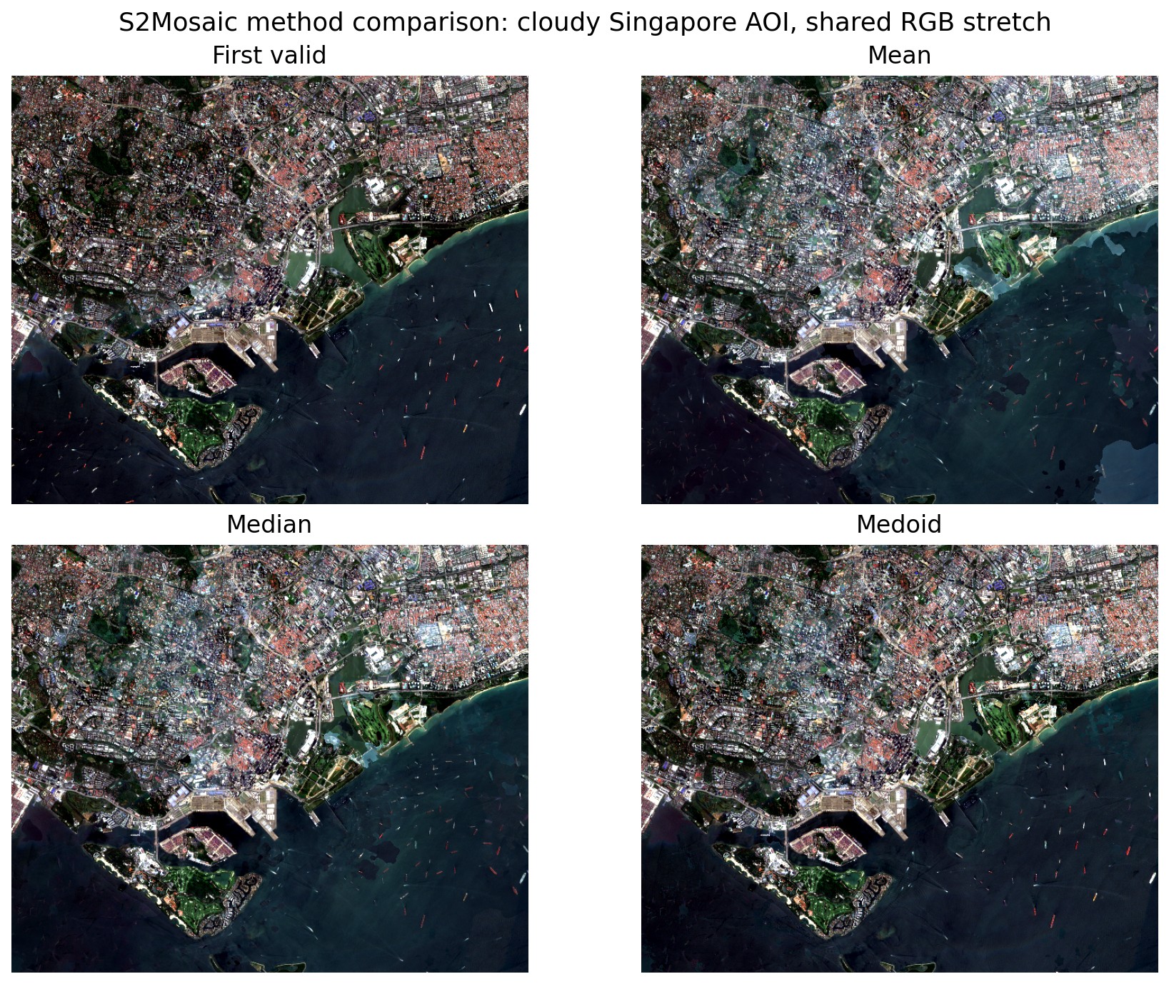
The image was generated by Mosaic method comparison.ipynb.
Advanced usage
Every mosaic() parameter, with defaults shown in parentheses.
Area (pass exactly one)
grid_id(None): Sentinel-2 MGRS tile ID, e.g."50HMH". Mosaics the entire tile.bounds(None):(minx, miny, maxx, maxy)rectangle. Mosaics an arbitrary AOI, including ones that cross MGRS tile boundaries. See the bounds/AOI-mode-specific options below.aoi(None): single shapelyPolygon. Mosaics the polygon bounds while skipping and masking pixels outside the polygon. Mutually exclusive withgrid_idandbounds.
Time window
start_year(required),start_month(1),start_day(1): start of the scene-search window.duration_years(0),duration_months(0),duration_days(0): length of the search window. Inclusive ofstart_*, exclusive of the end.
Output content
bands(["B04", "B03", "B02", "B08"]): bands to include. Leave asNoneto use the default RGB+NIR set. Use["visual"]for the 3-band uint8 TCI RGB composite (mutually exclusive with other bands).mosaic_method("mean"): how per-pixel scene stacks are reduced to one output value."mean": per-band arithmetic mean of all valid scenes. Streams scenes incrementally so peak memory stays small."first": first valid pixel inscene_order. The cheapest method. Reads only what's needed to fill each tile and stops as soon as it can."percentile": per-band percentile across all valid scenes. Requires thepercentileparameter (0-100)."median": shortcut for"percentile"withpercentile=50."medoid": picks the scene whose multi-band spectrum is closest (squared Euclidean) to the per-band median across all valid scenes for the pixel. Preserves real observed spectra, so band relationships stay coherent for indices and classifiers. This is the approximate-medoid formulation used by LandTrendr on Google Earth Engine (Kennedy et al. 2018) and the Open-MRV tutorials, not the strict Flood 2013 pairwise-distance medoid; the two often agree, but can differ.
percentile(None): percentile to compute whenmosaic_method="percentile"(0-100).min_observations(None): minimum valid observations to read per pixel for"mean","percentile", and"medoid". When set, tile aggregation stops reading later scenes once every coverable pixel has reached the target. This is not an output quality guarantee; pixels that cannot reach the target use whatever observations are available.max_observations(None): per-pixel cap on valid observations for"mean","percentile", and"medoid". Each pixel accepts at most this many scenes (inscene_order); later valid scenes are dropped for that pixel. Combined withscene_order="oldest"or"newest"this biases the mosaic toward early or late dates. Must be>= min_observationswhen both are set; ignored by"first"(effectively N=1).include_observation_count(False): append a finalObservation countband with the number of valid source scenes that contributed to each output pixel. Works for both returned arrays and exported GeoTIFFs. Forbands=["visual"], enabling this writes/returnsuint16output so the count band is not limited to 255; the RGB values remain in their usual 0-255 range.tile_workers(8): number of output tiles to aggregate concurrently. Tuned higher than CPU count because the work is I/O-bound on remote COG reads. Raise for faster networks; lower if memory or simultaneous-connection limits matter more than throughput.adaptive_tiling(True): split sparse output tiles based on the actual cloud-valid contribution masks. This reduces wasted reads for irregular AOIs, sparse coverage, and heavily masked scenes. Set toFalseto use fixed-size output tiles.
Output destination
output_dir(None): if set, writes a GeoTIFF to this directory using an auto-generated filename and returns the file path. The filename includes a readable request summary plus a short deterministic hash, and a matching.jsonsidecar records the normalized request metadata. Mutually exclusive withoutput_path.output_path(None): if set, writes a GeoTIFF to this exact.tif/.tiffpath and returns it. The.jsonsidecar is written here too, alongside the GeoTIFF. Mutually exclusive withoutput_dir.overwrite(True): when exporting and the target path exists, controls whether to overwrite it.
Output grid
output_crs(None): EPSG of the output. Must be a projected CRS. Geographic CRSes (e.g. 4326) are rejected at validation, becauseresolutionis metres in the target CRS and a geographic output would produce a degenerate grid. If you need a lat/lon raster, reproject the mosaic afterwards withgdalwarp/rio warp. In bounds/AOI mode, auto-picked as the UTM zone containing the AOI centroid if omitted. For AOIs wider than ~6° of longitude (one UTM zone), pass an explicit equal-area projection instead (e.g.output_crs=3577for Australia,5070for the contiguous US), because the auto-picked centroid UTM has growing scale distortion and a larger envelope overshoot far from its central meridian. Ignored in grid mode (the tile's native UTM zone is used).resolution(10): output pixel size in metres. Coarser resolutions read from the coarsest COG overview that is no coarser than the output pixel, in every mode, so much less data crosses the wire. Overviews are a fixed set of levels (MPC 2x-32x, AWS 2x-16x, DEA only 8x-32x); when a request falls well between them (at least 4x the pixels needed, e.g. 60 m from DEA's 10 m bands, which has no overview under 80 m), S2Mosaic logs a warning naming the nearest efficient resolutions. Each warning is shown once per session, so a loop ofmosaic()calls logs it once.resampling_method("nearest"): how the source is resampled to the output grid. Also accepts"bilinear","cubic","average","lanczos".snap_to_source_grid(False): bounds/AOI mode only. WhenTrue, expand the output extent outward to whole multiples ofresolutionin the target CRS. This makes repeat runs over the same area produce identical grids, and atresolution=10aligns the output to the native Sentinel-2 pixel grid, so source COG reads become zero-cost copies rather than sub-pixel resamples. The output may grow by up to one pixel on each side; pixels outside anaoipolygon are still written as nodata.
Scene selection
source("MPC"): STAC provider."MPC"(default) uses Microsoft Planetary Computer with SAS-signed URLs."AWS"uses Element 84's Earth Search on AWS Open Data: Sentinel-2 L2A scenes, public COGs, no auth, no SAS rotation."DEA"uses Digital Earth Australia's Sentinel-2 NBART (Australia only; see Choosing a source). All return spectral bands on one scale,reflectance * 10000: from processing baseline 04.00 (January 2022) ESA adds 1000 to every spectral DN, Element 84 removes it before publishing, and S2Mosaic removes it from MPC scenes at read time. A 04.00+ DN at or below 1000 (reflectance <= 0, e.g. dark water) reads as 1, not 0, so it stays a valid observation; 0 is always nodata.additional_query({"eo:cloud_cover": {"lt": 100}}): extra STAC query filters in the Query extension's form, e.g.{"eo:cloud_cover": {"lt": 80}}. DEA's API only accepts CQL2, so forsource="DEA"the filter is translated; the operatorseq,neq,lt,lte,gt,gteandinare supported, and any other raises instead of being dropped. Property names are the provider's own (DEA's cloud cover is fmask's, aseo:cloud_cover).min_coverage_fraction(None): optional scene-edge trimming. When set, drops pixels covered by fewer than this fraction of the maximum scene-overlap count in the requested area. The default keeps the full requested coverage.ignore_duplicate_items(True): drop duplicate acquisitions, keeping the latest processing baseline.
Scene ordering
scene_order("valid_data"): scene ordering. One of"valid_data","oldest", or"newest".scene_sort_fn(None): custom callablefn(items: pd.DataFrame) -> pd.DataFrame. Overridesscene_orderwhen set.
Cloud masking
cloud_mask("OCM"): mask provider."OCM"runs the OmniCloudMask deep-learning model on R+G+NIR bands (most accurate);"SCL"reads the L2A Scene Classification Layer (much cheaper, lower accuracy). Onsource="DEA", which has no SCL,"SCL"reads DEA's fmask layer.ocm_batch_size(1): OCM inference batch size. Only used withcloud_mask="OCM".ocm_inference_dtype("fp32"): OCM inference dtype. Defaults to"fp32", which runs everywhere and is the fastest option on CPU. On GPU, use"fp16"for ~2× speedup and lower VRAM, or"bf16"on hardware that supports it. Only used withcloud_mask="OCM".
Diagnostics
show_progress(False): show tqdm progress bars for the cloud-mask streaming and tile-aggregation phases. Useful in notebooks; leave off for headless/batch runs.
Example:
array, profile = mosaic(
    bounds=(389410, 6462290, 397010, 6465700),
    input_crs=32750,
    snap_to_source_grid=True,
    start_year=2023,
    duration_months=2,
    bands=["visual"],
    mosaic_method="mean",
    include_observation_count=True,
)

rgb = array[:3]
observation_count = array[3]
print(array.shape)  # (4, height, width): Red, Green, Blue, Observation count
Bounds/AOI-mode-specific options
input_crs(4326): EPSG ofboundsoraoi.
For the exact function signature and return types, see the mosaic() docstring in the source code.
Logging
S2Mosaic emits progress logs at each pipeline stage (search, sort, fetch, cloud-mask, aggregate, export). Following standard Python logging convention, no output is produced unless logging is configured. The simplest way to enable it:
import s2mosaic

s2mosaic.set_log_level("INFO")  # or "DEBUG" for more detail
If your application already configures the logging module, the package logger (s2mosaic) will respect that, and there is no need to call set_log_level().
Performance tips
cloud_mask: Default"OCM"runs the OmniCloudMask deep-learning model, which is the most accurate but needs reasonable compute (GPU/MPS recommended). Switch to"SCL"on CPU-only machines or for bulk processing; it skips inference entirely and just reads the L2A Scene Classification Layer.ocm_batch_size: If using a GPU, setting this above the default value (1) will speed up cloud masking. In most cases, a value of 4 works well. If you encounter CUDA errors, try using a lower number.ocm_inference_dtype: defaults to'fp32', which runs on every backend and is the fastest option on CPU (most CPUs don't have efficient fp16/bf16 paths). On GPU, switch to'fp16'for ~2× faster inference and lower VRAM use, or'bf16'on hardware that supports it (Ampere+ NVIDIA, Apple Silicon).scene_order: Using"valid_data"tends to work well with early stopping because clear scenes are considered first.min_observations: For large"mean","percentile", or"medoid"jobs, set this to the number of observations per pixel you actually need to avoid reading later scenes for already-satisfied tiles.max_observations: Caps each pixel at N valid scenes. Combine withscene_order="oldest"(or"newest") to bias the mosaic toward early/late dates over a long search window without paying for the extra reads.resolution: Data read scales with the source level each read comes from, not just the output size. Resolutions that land on a COG overview (native, or 2x, 4x, 8x... of it; DEA only has 8x and coarser) read the least; ones between levels read the finer level and downsample. S2Mosaic warns when that costs 4x or more.mosaic_method: Roughly ordered fastest to slowest,"first"<"mean"<"percentile"/"median"≈"medoid"."first"only reads pixels needed to fill each tile and stops as soon as it can, so cloud-free scenes can finish a tile in one pass."mean"streams every contributing scene but accumulates incrementally, so its memory stays small."percentile"/"median"and"medoid"both hold each tile's per-scene stack in memory to compute the result, so they use more RAM and, withoutmin_observations/max_observations, read every contributing scene. Both keep that stack asuint16plus a separate validity mask, so it is the same size for either method."medoid"still peaks lower because its kernel returnsuint16directly and stripe-blocks its scratch arrays, while percentile/median returnsfloat32and is clipped back afterwards: on a 12-scene, 4-band, 2048px tile the stack is 403 MB and peak is roughly 690 MB for median against 540 MB for medoid. Peak scales with scene count (the same tile over 34 scenes peaks at about 1.5 GB) and every tile worker pays it, sotile_workersmultiplies it. Setmin_observations(and/ormax_observations) to cap reads once every coverable pixel has enough samples.
Known limitations
-
SCL is less accurate than OCM. The L2A Scene Classification Layer is fast (one COG read per scene, no inference) but is consistently less accurate than OCM at identifying clouds and cloud shadow. Use SCL when compute is the bottleneck (CPU-only machines, bulk processing); use OCM when accuracy matters.
-
Microsoft Planetary Computer serves isolated single-band zeros over dark water. At roughly 0.01-0.04% of valid pixels, one band reads
0(NODATA) where its neighbours read near-zero reflectance. On the harmonised scale (seesource) the value is off by only a few DN, but a zero in one band still distorts ratios and spectral indices at those pixels, where the denominators are already small. A pixel is only discarded when every requested band reads 0, so these survive: discarding them instead would throw away the good bands to avoid the bad one, and leave a hole no other scene could fill. Element 84's copy of the same acquisitions is unaffected, sosource="AWS"avoids it entirely. -
bands=["visual"]cannot distinguish black water from no data. TCI is a quantised 8-bit render, so near-zero reflectance rounds to 0, and ESA also reserves 0 for NODATA. A pixel whose three channels all round to 0 is therefore indistinguishable from an unobserved one and is dropped - about 0.23% of valid pixels on a Perth AOI, all inside water that renders near black anyway. Request the spectral bands instead where dark water matters, since there DN 0 really is NODATA. -
source="DEA"lags about two weeks and drops a few scenes. Onlyfinaldatasets are searched, and a final version usually appears 9-13 days after acquisition (up to ~50), so a window ending in the last couple of weeks has fewer scenes than on MPC or AWS. A small number of acquisitions (1-3 per tile over April-September 2026 on three sampled tiles) are only ever published as provisionalnrt, and are never included. DEA also publishes novisualasset; request["B04", "B03", "B02"]and stretch for display.
Contributing
Contributions are welcome. Open an issue or a pull request.
Running the tests
Tests use pytest. The development environment uses the Python pinned in .python-version (3.14); CI runs the suite on every supported version, 3.10-3.14. The fast suite (unit tests + mocked pipelines) takes well under a minute and is what CI runs by default:
uv run pytest                       # full fast suite
uv run pytest tests/test_readers.py # one file
uv run pytest -k requeue            # match by name
End-to-end tests that hit the network and run a real mosaic are marked slow and excluded by default (see addopts in pyproject.toml). To run them explicitly:
uv run pytest -m slow               # only slow tests
uv run pytest -m ""                 # everything, including slow
The example notebooks run against live STAC sources and take several minutes, so they are not part of the per-push CI. A separate workflow executes them weekly, on pull requests that change examples/, and on demand from the Actions tab. To run them locally:
uv run pytest --nbmake examples/*.ipynb
Lint with ruff:
uv run ruff check s2mosaic/ tests/
For maintainers: the release flow (cut a tag, GitHub Actions builds + publishes to PyPI) is documented in RELEASING.md.
License
This project is licensed under the MIT License.
Acknowledgments
S2Mosaic is built on top of:
- Sentinel-2: ESA's Copernicus Earth-observation mission, the imagery source.
- Element 84 Earth Search: optional public AWS Open Data access to Sentinel-2 L2A COGs.
- Microsoft Planetary Computer: the default STAC catalog and signed access to the Sentinel-2 L2A archive.
- Digital Earth Australia: Geoscience Australia's Sentinel-2 NBART analysis-ready data and fmask, used by
source="DEA". - OmniCloudMask: the deep-learning cloud and cloud-shadow mask used by the default
cloud_mask="OCM"provider. - L2A Scene Classification Layer (SCL): the published per-scene classification used by the optional
cloud_mask="SCL"provider. - rasterio, GeoPandas, pystac-client, OpenCV, Numba, and multiclean: supporting libraries for I/O (including per-scene
WarpedVRTreprojection), geometry, search, image ops, percentile aggregation, and mask post-processing.
1 maintainer

Metadata
1 maintainer
Release files for s2mosaic 2.0.0b6
For a detailed explanation of source distributions (sdists) and built distributions (wheels), please see the package formats documentation.
Source distribution (sdist)
| File | Size | Uploaded | |
|---|---|---|---|
| s2mosaic-2.0.0b6.tar.gz | 9.7 MB | Details |
Built distribution (wheel)
| File | Interpreter | ABI | Platform | Reset |
|---|---|---|---|---|
| s2mosaic-2.0.0b6-py3-none-any.whl | Python 3 | none | any | Details |
Total release size: 9.8 MB
Release files / s2mosaic-2.0.0b6.tar.gz
| Download URL | s2mosaic-2.0.0b6.tar.gz |
|---|---|
| Size | 9.7 MB |
| Tags | Source |
|
SHA-256 checksum How to use checksums |
1f30073b0b298e11ba151738a560f67906144c1f500ff3b6be68df1e7103d622
|
|
BLAKE2b-256 checksum How to use checksums |
6a585396ec9a047fe0961c63b5f021e3171aca32fbcf2b5764e2c89ed3d01487
|
| Upload date | |
|
Uploaded using Trusted Publishing? What is trusted publishing? |
Yes |
| Uploaded via |
twine/7.0.0 CPython/3.13.14
|
Provenance
Provenance describes where a file came from. On PyPI, provenance is shared via attestations, which provide a verifiable record of the build or publishing details. View details, limitations and caveats.


PyPI Publish Attestation
PyPI verified that this artifact, at this checksum, originated from the publisher listed below.
Signed by GitHub Actions, verified by PyPI on Oct 5, 2026.
Transparency logRelease files / s2mosaic-2.0.0b6-py3-none-any.whl
| Download URL | s2mosaic-2.0.0b6-py3-none-any.whl |
|---|---|
| Size | 106.4 kB |
| Tags | Python 3 |
|
SHA-256 checksum How to use checksums |
115b4877998843cb1b1f3c6aaf23af9937c33a63cf0fa8a9f77ab945b5014c6f
|
|
BLAKE2b-256 checksum How to use checksums |
b58339cfcdb16099c553d1607af81f04405f5063df1fbac035be28e3188a57b8
|
| Upload date | |
|
Uploaded using Trusted Publishing? What is trusted publishing? |
Yes |
| Uploaded via |
twine/7.0.0 CPython/3.13.14
|
Provenance
Provenance describes where a file came from. On PyPI, provenance is shared via attestations, which provide a verifiable record of the build or publishing details. View details, limitations and caveats.
PyPI Publish Attestation
PyPI verified that this artifact, at this checksum, originated from the publisher listed below.
Signed by GitHub Actions, verified by PyPI on Oct 5, 2026.
Transparency log













