
SaMoVAR
Structural Aligned Mixture of VAR — a linear-attention Transformer that is a dynamic VAR model.
A documented Python implementation of Lu & Yang (2025), Linear Transformers as VAR Models: Aligning Autoregressive Attention Mechanisms with Autoregressive Forecasting (ICML 2025, PMLR 267, arXiv:2502.07244), rebuilt as a library for applied econometric work: fit, forecast, benchmark against classical VAR/AR baselines, and read the implied lag matrices, impulse responses and influence paths back out of the trained network.
Maintainer: Dr Merwan Roudane — merwanroudane920@gmail.com — https://github.com/merwanroudane
pip install samovar-var # import samovar
Documentation
| 📘 User guide | Task-oriented cookbook: 16 sections of copy-paste syntax — loading data, choosing the horizon, training, forecasting, benchmarking, interpretation, figures, LaTeX tables, production use, field-specific recipes |
| 📊 Every output, in full | What each example prints and writes — console logs, every table, every figure, with the numbers you should reproduce |
| 🧮 Theory & paper mapping | The derivation, the mapping to each equation of the paper, and the complete list of differences between the paper, the authors' released code and this implementation |
| 🧪 Examples | Five runnable scripts, from a 1-minute quickstart to a full ablation study |
| 📄 Paper | Lu & Yang (2025), ICML — the method this library implements |
Table of contents
- Why this model
- Installation
- Sixty-second tour
- The method in one page
- Choosing
horizonandinput_length - Full API reference
- Working with your own data
- Interpretation: getting the VAR out
- Benchmarking and tests
- Tables and figures for a paper
- Worked examples
- Reproducing the paper's design choices
- Troubleshooting
- Citation and license
Companion documents: docs/GUIDE.md — a task-oriented
cookbook ("how do I write the code for X"), and
docs/THEORY.md — the derivation, the mapping to every
equation of the paper, and the complete list of differences between the paper,
the authors' released code and this implementation.
1. Why this model
A single causal linear-attention layer, written out, is
$$o_t^\top ;=; \sum_{i\le t} \mathbf{A}{t,i},k_i^\top, \qquad \mathbf{A}{t,i} = v_i^\top q_t$$
which is exactly a VAR($t$) with data-dependent lag matrices: the keys are the observations and the rank-1 outer products $v_i^\top q_t$ are the coefficients, regenerated at every time step. Standard Transformer plumbing (residual streams, interleaved MLPs, key projections) destroys that structure. SaMoVAR rearranges the architecture so it survives stacking, which buys three things at once:
| Accuracy | Wins on 12 standard forecasting benchmarks in the original paper (avg. rank 1.41 vs 2.86 for the next best) |
| Interpretability | The fitted network is a time-varying VAR — you can extract $A_1,\dots,A_p$, impulse responses, and the exact paths through which past shocks reach the forecast |
| Cost | $O(L)$ in sequence length, no key-projection matrix, one shared output matrix — smaller and cheaper than a plain linear Transformer |
What this library adds on top of the paper: a scikit-learn-style estimator, classical econometric baselines (AR, VAR, ridge, naive), Diebold–Mariano tests, exact coefficient recovery (validated by a unit test against the network's own forward pass), impulse responses, publication-quality figures and LaTeX tables, and economic datasets ready to load.
2. Installation
pip install samovar-var
The distribution is samovar-var; the import is samovar (the plain samovar
name on PyPI belongs to an unrelated project).
From source, to get the examples and tests as well:
git clone https://github.com/merwanroudane/SaMoVAR.git
cd SaMoVAR
pip install -e ".[all]"
Requirements: Python ≥ 3.9, torch ≥ 2.0, numpy, pandas, scipy, matplotlib, statsmodels. A GPU is optional — every example in this README runs on a laptop CPU in minutes.
Check the install:
python -c "import samovar; print(samovar.__version__)"
pytest -q                     # 26 tests, ~20 s
3. Sixty-second tour
import pandas as pd
from samovar import SaMoVAR
from samovar.datasets import load_us_macro

df = load_us_macro()          # 202 quarters x 6 US macro series, ships offline

model = SaMoVAR(
    horizon=4,                # forecast 4 quarters == one patch
    input_length=32,          # read 8 years of history == 8 patches
    n_layers=3,
    epochs=150,
)
model.fit(df)

model.forecast()              # DataFrame, 4 rows, future dates as index
model.evaluate()              # {'MSE': ..., 'MAE': ..., 'RMSE': ..., 'R2': ..., 'MASE': ...}
model.compare()               # accuracy table vs naive / AR / VAR / ridge
model.var_coefficients()      # implied VAR lag matrices at the last origin
model.impulse_response(12)    # dynamic multipliers, (13, C, C)
model.save("macro.pt")
Every method is documented below, and model.summary() prints the resolved architecture:
SaMoVARConfig
  series (C)            : 6
  input length (L_I)    : 32  (+0 pad)
  horizon / patch (L_P) : 4
  patches (N)           : 8
  tokens (2N)           : 16
  width (d)             : 64 = 4 heads x 16
  layers (l)            : 3
  ARX tokenisation      : True
  structural matrix D   : direct (shortcut inside: False)
  key projection W_k    : False
  QV RMSNorm            : True
  instance norm         : last_patch
  AR loss weight        : 1.0
  parameters            : 63,428
Defaults follow the authors' released implementation, not the (slightly
different) equations printed in the paper — see §12 for the switches that flip
each one back, and docs/THEORY.md §6 for the full list of differences.
4. The method in one page
Tokenisation (ARX). The input window is front-padded and cut into $N$ non-overlapping patches of length $L_P$ = the forecast horizon. Each series $j$ gets an endogenous token $W_{tok},S^{[i:i+L_P,j]}$, preceded by an exogenous token built from all series through $W_{ex}\in\mathbb{R}^{C\times C}$. The sequence a channel sees is [ex₁, en₁, ex₂, en₂, …] — a VARX system in patch time. The channel axis is folded into the batch, so parameter count does not grow with $C$.
Representation. All $l$ MLP blocks run first and produce the VAR observation $x^{(1)}$, followed by RMSNorm. No MLP is interleaved between attention layers — that is what would break the VAR recursion.
VAR stack. Layer $m$ takes keys from the previous layer's output ($k^{(m)} = o^{(m-1)}$, no $W_k$) and queries/values from the first-layer input $x^{(1)}$, each RMSNorm'd per head. Composing layers gives
$$\mathbf{B}^{(m)}{t,j} ;=; \sum{i=j}^{t}\big(v^{(m)\top}i q^{(m)}t\big),\mathbf{B}^{(m-1)}{i,j},\qquad \mathbf{B}^{(0)}{i,j} = \mathbf{I},\mathbb{1}_{[i=j]}$$
Mixture + shortcut + structure. Outputs of all layers are summed, multiplied by an invertible per-head matrix $\mathbf{D}$ in LU form, and the observation itself is added back (the "key shortcut", the $l=0$ path):
$$\hat{x}^{(1)\top}{t+1} ;=; x_t^{(1)\top} ;+; \sum{j\le t}\mathbf{D}\Big(\sum_{m=1}^{l}\mathbf{B}^{(m)}_{t,j}\Big) x_j^{(1)\top}$$
That is what the released code computes (generate_S(get_inverse=False), identity added after the transform), and it is the default here. The paper writes the equivalent structural form $\hat{x}{t+1}=\sum_j \mathbf{D}^{-1}\mathbf{C}{t,j}x_j$ with $\mathbf{C}{t,j}=\sum_m\mathbf{B}^{(m)}{t,j}+\mathbf{I}\mathbb{1}_{[j=t]}$; pass structural_matrix="inverse", shortcut_in_structural=True for that reading.
Temporal influence paths. Expanding $\mathbf{C}{t,j}$ gives one term per weakly ordered chain $t \ge i_1 \ge \dots \ge i{m-1} \ge j$, with magnitude equal to a product of dot products across layers. The number of paths is $1+\sum_{m=1}^{l}\binom{(t-j)+(m-1)}{m-1}$ — SaMoVARConfig.n_paths(lag) computes it. This is where interpretability comes from: you can ask through which intermediate dates a shock in 2008Q3 reaches the forecast for 2010Q1.
Loss. Terminal forecasting MSE + a next-patch autoregressive MSE applied at every position (weight ar_loss_weight).
Full derivation, with the mapping to each equation of the paper and the list of places where this implementation deviates from the authors' reference code: docs/THEORY.md.
5. Choosing horizon and input_length
These two numbers matter more than anything else.
horizon= the patch size = what you forecast in one shot. Pick the horizon you actually care about: 4 or 8 for quarterly, 12 for monthly, 24 for hourly. Do not set it to 1 unless you want observation-level lag matrices (useful for interpretation, expensive for long windows).input_lengthshould be a multiple ofhorizon(it is front-padded otherwise) and give you 8–12 patches. The paper uses ratios of roughly 6:1 to 11:1.
| Frequency | horizon |
input_length |
patches | tokens |
|---|---|---|---|---|
| Quarterly, 1 year ahead | 4 | 32–48 | 8–12 | 16–24 |
| Monthly, 1 year ahead | 12 | 96–144 | 8–12 | 16–24 |
| Daily, 1 month ahead | 21 | 168–252 | 8–12 | 16–24 |
| Hourly, 1 day ahead | 24 | 192–336 | 8–14 | 16–28 |
Minimum sample size: you need input_length + horizon observations for a single window. For training you want at least a few hundred windows, i.e. roughly input_length + horizon + 300 observations. Below ~250 observations, a classical VAR is usually the better tool — the library ships one so you can check.
6. Full API reference
6.1 SaMoVAR — the estimator
SaMoVAR(
    horizon,                      # int   L_P: forecast length AND patch size
    input_length,                 # int   L_I: history length
    *,
    # --- architecture -------------------------------------------------
    n_layers=3,                   # int   l: MLP layers and attention layers
    d_model=None,                 # int   width; default 32*floor(sqrt(C)) snapped to head_dim
    head_dim=16,                  # int   per-head width (paper pins this at 16)
    n_heads=None,                 # int   overrides d_model // head_dim
    dropout=0.1,
    mlp_ratio=4,
    exogenous=True,               # bool  ARX tokenisation (cross-series stream)
    structural_matrix="inverse",  # "inverse" | "direct" | "none"
    shortcut_in_structural=True,  # bool  identity term passes through D
    use_key_projection=False,     # bool  ablation: re-introduce W_k
    qv_norm=True,                 # bool  RMSNorm on queries and values
    predictor="dynamic",          # "dynamic" | "fixed" (FixedVAR control model)
    ar_loss_weight=1.0,           # float weight of the next-patch loss
    normalization="revin",        # "revin" | "last_patch" | "none"
    # --- optimisation -------------------------------------------------
    epochs=100, batch_size=32, lr=6e-4, weight_decay=0.1,
    patience=12, max_grad_norm=1.0, accumulation_steps=1, warmup_pct=0.05,
    amp=False, num_workers=0,
    # --- data ---------------------------------------------------------
    scale=True, val_ratio=0.1, test_ratio=0.2, stride=1,
    # --- misc ---------------------------------------------------------
    device=None, seed=2024, verbose=1, checkpoint_dir=None,
)
Fitting
| Method | Signature | Returns |
|---|---|---|
fit |
fit(data, validation_data=None, callbacks=None) |
self |
data is a DataFrame (ideally with a DatetimeIndex) or a (T, C) array. Without validation_data the sample is split chronologically 1-val_ratio-test_ratio / val_ratio / test_ratio; the scaler is fitted on the training block only. callbacks are callable(epoch, logs).
Forecasting
| Method | Signature | Returns |
|---|---|---|
predict |
predict(data=None, as_frame=True) |
one-shot horizon-step forecast |
forecast |
forecast(steps=None, data=None, as_frame=True) |
steps ahead, rolling forward recursively if steps > horizon |
predict_windows |
predict_windows(windows, scaled_input=True, return_scaled=True, batch_size=64) |
(n, L_P, C) for a batch of windows |
model.predict()                       # next 4 quarters, original units, dated index
model.forecast(steps=12)              # 12 steps by recursion
model.predict(data=other_df)          # apply the fitted model to a different panel
model.predict_windows(X, scaled_input=False, return_scaled=False)
Evaluation
| Method | Signature | Returns |
|---|---|---|
evaluate |
evaluate(data=None, split="test", per_series=False, seasonality=1) |
dict of MSE, MAE, RMSE, sMAPE, R², MASE |
backtest |
backtest(data=None, split="test", return_predictions=False) |
per-origin DataFrame |
error_by_horizon |
error_by_horizon(split="test", metric="MSE") |
(horizon,) array |
compare |
compare(models=None, split="test", metrics=("MSE","MAE","RMSE")) |
benchmark table |
residual_covariance |
residual_covariance(split="train") |
(C, C) |
model.evaluate(per_series=True)                 # metrics per series
per_origin = model.backtest()                   # rolling-origin MSE/MAE
table = model.compare()                         # vs naive/AR/VAR/ridge
table = model.compare([VARForecaster(4), ARForecaster(4, 8)])   # your own list
Interpretation
| Method | Signature | Returns |
|---|---|---|
var_coefficients |
var_coefficients(data=None, origin=-1, max_lags=None, reduce="mean", as_frame=False) |
dict with A (p, C, C), or tidy DataFrame |
coefficient_paths |
coefficient_paths(split="test", max_lags=None, max_origins=60) |
draws, mean, std, lo, hi |
impulse_response |
impulse_response(horizon=12, shock="unit"|"cholesky"|"custom", sigma=None, cumulative=False) |
(H+1, C, C) |
influence_paths |
influence_paths(source_lag=4, series=0, top_k=8) |
list of paths with weights |
attention_map |
attention_map(series=0, layer=None) |
(T, T) lower-triangular |
contribution_profile |
contribution_profile(series=0) |
own vs cross contribution by lag |
token_labels |
token_labels() |
{index: "t-3\n(Ex)"} for figures |
Persistence
model.save("model.pt")               # weights + config + scaler + last window
model = SaMoVAR.load("model.pt")     # ready to forecast
6.2 Modules
| Module | What is in it |
|---|---|
samovar.config |
SaMoVARConfig, TrainConfig — serialisable, with .summary(), .save(), .load() |
samovar.model |
SaMoVARNet, LinTransNet, build_network(cfg, "samovar"|"lintrans"|"fixedvar") |
samovar.layers |
LinearVARAttention, FixedVARAttention, StructuralMatrix, RMSNorm, MLP |
samovar.tokenizer |
ARXTokenizer, InstanceNorm |
samovar.data |
prepare_data, WindowDataset, sliding_windows, simulate_var, StandardScaler |
samovar.datasets |
load_us_macro, load_fred_md, load_interest_inflation, load_csv, load_simulated_var, describe |
samovar.trainer |
Trainer, History |
samovar.baselines |
NaiveForecaster, SeasonalNaive, MeanForecaster, ARForecaster, VARForecaster, RidgeDirect |
samovar.metrics |
mse, mae, rmse, mape, smape, mase, r2_score, direction_accuracy, all_metrics, diebold_mariano |
samovar.interpret |
mixture_weights, lag_matrices, var_coefficients, average_var_coefficients, temporal_influence_paths, impulse_response, attention_map, contribution_profile |
samovar.plotting |
12 figure functions, all returning a Figure |
samovar.report |
to_latex, to_markdown, save_table, ranking_table, dm_matrix |
samovar.style |
set_style, parula_colors, parula_cmap, diverging_cmap, savefig |
7. Working with your own data
7.1 The shape contract
One row per time stamp, one column per series, no missing values, sorted ascending:
import pandas as pd
df = pd.read_csv("my_data.csv", parse_dates=["date"]).set_index("date").sort_index()
df = df.dropna()                    # or interpolate first
model = SaMoVAR(horizon=12, input_length=120).fit(df)
samovar.datasets.load_csv does this for you:
from samovar.datasets import load_csv
df = load_csv("my_data.csv", date_column="date", freq="MS")
7.2 Stationarity
SaMoVAR normalises each window internally (RevIN), which removes level and scale but not a unit root's persistence. Treat it like any VAR: difference or log-difference first, and keep rates in levels.
import numpy as np
work = pd.DataFrame({
    "gdp_growth": 100 * np.log(df["gdp"]).diff(),
    "inflation":  100 * np.log(df["cpi"]).diff(),
    "policy_rate": df["rate"],              # a rate: keep the level
}).dropna()
samovar.datasets.describe(df) gives you the descriptive table with ADF statistics to justify the choice.
7.3 Exogenous variables and target subsets
Every column is both a predictor and a target. To use a variable without forecasting it, include it in df and simply ignore its column in the output. To turn the cross-series channel off entirely (pure univariate AR on each series), pass exogenous=False.
7.4 Panels with many series
The channel axis is folded into the batch, so 100+ series work — but memory scales with batch_size × C. Reduce batch_size and raise accumulation_steps to keep the effective batch:
SaMoVAR(horizon=12, input_length=120, batch_size=8, accumulation_steps=4) # effective 32
(Unlike the reference implementation, accumulation here really accumulates — see docs/THEORY.md.)
8. Interpretation: getting the VAR out
This is the part a classical Transformer cannot give you.
8.1 Lag matrices
coefs = model.var_coefficients(max_lags=6, reduce="mean")
A = coefs["A"]                 # (6, C, C): A[k][i, j] = effect of series j at lag k+1 on series i
coefs["lags"]                  # [1, 2, 3, 4, 5, 6]  measured in patches of `horizon` steps
Two routes are available through method=:
method |
What it is | Units | Use it for |
|---|---|---|---|
"jacobian" (default) |
exact Jacobian $\partial\hat y_{T+h}/\partial y_{T-k}$ of the whole network | data units, comparable with a classical VAR's $A_k$ | anything you report |
"algebraic" |
the model's own token-space decomposition $\mathbf{D}\sum_m\mathbf{B}^{(m)}$, split into an endogenous and an exogenous part | token space, scale not calibrated | attributing an effect to own-lag vs cross-series, to a layer, or to a path |
The Jacobian route is exact because the network's only non-linearities are GELU
and the normalisations: around any window it is a linear map, and that map is a
VAR. With horizon=1, A[k-1][c, s] is literally
$\partial\hat y_{t+1,c}/\partial y_{t+1-k,s}$.
Lag $k$ means "$k$ patches back", i.e. $k \times$ horizon observations. Set horizon=1 if you want observation-level lags — then A[k-1][c, s] is exactly $\partial\hat y_{t+1,c}/\partial y_{t+1-k,s}$, the same object a classical VAR reports.
With horizon > 1 each lag carries an $L_P \times L_P$ block, and reduce decides how it is collapsed. This changes the magnitude — state your choice in the table caption:
reduce |
Meaning | Rough magnitude |
|---|---|---|
"mean" (default) |
average marginal effect of one observation of the source patch on one observation of the forecast | classical coefficient ÷ $L_P$ |
"sum" |
total effect of the whole source patch on the whole forecast | comparable to a cumulated multiplier |
"trace" |
effect of step $u$ of the source on step $u$ of the forecast, averaged over $u$ | same-step effect |
"last" |
last observation of the patch → last forecast step | one specific cell |
"none" |
keep the full $(L_P, L_P)$ blocks | — |
Tidy form for regression tables:
model.var_coefficients(max_lags=4, as_frame=True).head()
#    lag response  shock  coefficient
# 0    1      gdp    gdp        0.412
# 1    1      gdp    cpi       -0.087
8.2 They are exact, and there is a test that proves it
tests/test_core.py::test_mixture_weights_reproduce_the_forward_pass reconstructs the network's own output from the recovered token-space coefficients and asserts agreement to 1e-8 in double precision. The recursion is run with the real rank-1 matrices, in the same order as the forward pass (including where the key shortcut sits relative to $\mathbf{D}$). The Jacobian route is exact by construction.
8.3 Time-varying coefficients
The lag matrices are regenerated at every forecast origin — that is the model. To see the variation:
paths = model.coefficient_paths(split="test", max_lags=4, max_origins=120)
paths["mean"], paths["std"], paths["lo"], paths["hi"]     # (n_lags, C, C)
paths["draws"]                                            # (n_origins, n_lags, C, C)

from samovar.plotting import plot_coefficient_paths
plot_coefficient_paths(paths["draws"], lag=1, names=df.columns)
A classical VAR reports std == 0 here by construction.
8.4 Impulse responses
sigma = model.residual_covariance()
psi = model.impulse_response(horizon=12, shock="cholesky", sigma=sigma)   # (13, C, C)

from samovar.plotting import plot_irf
plot_irf(psi, names=df.columns, step_label="quarters (patches)")
Read this before you publish an IRF. $\mathbf{D}$ is an unrestricted LU factor learned by gradient descent — it is not an economic identification scheme. No short-run zeros, no long-run restrictions, no sign restrictions, no external instrument. What you get are model-implied dynamic multipliers of the estimated reduced-form dynamic VAR. Use
shock="cholesky"with an ordering you can defend, or supply your ownP, and describe the result as descriptive rather than structural.
8.5 Temporal influence paths
Through which intermediate dates does a past observation reach the forecast?
paths = model.influence_paths(source_lag=4, series=0, top_k=8)
paths[0]
# {'nodes': (12, 15, 19), 'layers': (1, 3), 'weight': -0.0412, 'n_layers': 2}

from samovar.plotting import plot_influence_paths
plot_influence_paths(paths, top_k=6, node_labels=model.token_labels())
nodes are token indices (source first); model.token_labels() maps them to t-3 (Ex) / t-1 (En) labels. A path that runs through (Ex) nodes is cross-series transmission; a path through (En) nodes only is own-series propagation.
weight is a relative magnitude in token space (a product of unnormalised query–value dot products), so rank and compare paths against each other — do not read a path weight as a regression coefficient. For data-unit magnitudes use var_coefficients.
8.6 Contribution decomposition and attention maps
model.contribution_profile(series=0)     # {"endogenous": ..., "exogenous": ..., "lags": ...}
model.attention_map(series=0)            # standardised q·k scores, lower triangular
9. Benchmarking and tests
from samovar.baselines import VARForecaster, ARForecaster, RidgeDirect, NaiveForecaster

table = model.compare([
    NaiveForecaster(4),
    ARForecaster(4, lags=4),
    VARForecaster(4, maxlags=8, ic="aic"),
    RidgeDirect(4, lookback=32),
])
Baselines are estimated on the same training block and evaluated on the same windows, so the comparison is like-for-like. Then test the difference:
from samovar.metrics import diebold_mariano
store = model._last_comparison
diebold_mariano(store["true"], store["pred"]["SaMoVAR"], store["pred"]["VAR(4)"], horizon=4)
# {'stat': -2.31, 'p_value': 0.021, 'mean_loss_diff': -0.043, 'n': 118}
Negative statistic ⇒ the first forecast has lower loss. The Harvey–Leybourne–Newbold small-sample correction and a Newey–West window of horizon - 1 lags are applied by default. For a full pairwise grid: samovar.report.dm_matrix(y_true, predictions_dict, horizon=4).
Across several datasets or horizons, samovar.report.ranking_table({...}) reproduces the paper's average-rank / top-1 summary.
10. Tables and figures for a paper
Tables
from samovar.report import to_latex, to_markdown, save_table

print(to_markdown(table[["MSE", "MAE"]]))                 # best bold, second underlined
tex = to_latex(table, caption="Out-of-sample accuracy.", label="tab:acc",
               note="Rolling origins over the last 20\\% of the sample.")
save_table(table, "assets/accuracy", caption="...", label="tab:acc")   # .tex + .md + .csv
The LaTeX output uses booktabs (\toprule/\midrule/\bottomrule) and, with note=, threeparttable.
Figures
from samovar import set_style
set_style("paper")        # or "talk", "poster"
| Function | Figure |
|---|---|
plot_history(history) |
training / validation curves with the best epoch marked |
plot_forecast(context, truth, prediction) |
one series with history, realisation, forecast |
plot_forecast_panel(...) |
small multiples, one panel per series |
plot_lag_matrices(A, names) |
grid of $C\times C$ coefficient heatmaps, one per lag |
plot_coefficient_heatmap(A, target=i) |
lag × source heatmap feeding one series |
plot_irf(psi, names, bands=(lo, hi)) |
impulse-response grid |
plot_influence_paths(paths) |
arc diagram of temporal influence paths |
plot_attention_map(matrix) |
causal $q_t\cdot k_i$ heatmap |
plot_contribution_profile(profile) |
own vs cross-series contribution by lag |
plot_error_by_horizon(errors) |
error as a function of the forecast step |
plot_benchmark(table, metric) |
ranked bar chart |
plot_ablation(table) |
% change vs the full model |
plot_coefficient_paths(draws, lag) |
coefficient time variation |
Colour maps: parula_cmap() (MATLAB Parula, from its 64 RGB stops), diverging_cmap() (blue–white–red, zero-centred), and a colour-blind-safe categorical PALETTE. Save with savefig(fig, "assets/name") → writes .pdf and .png at 300 dpi with pdf.fonttype=42 (editable text in Illustrator).
10b. What to expect: measured results
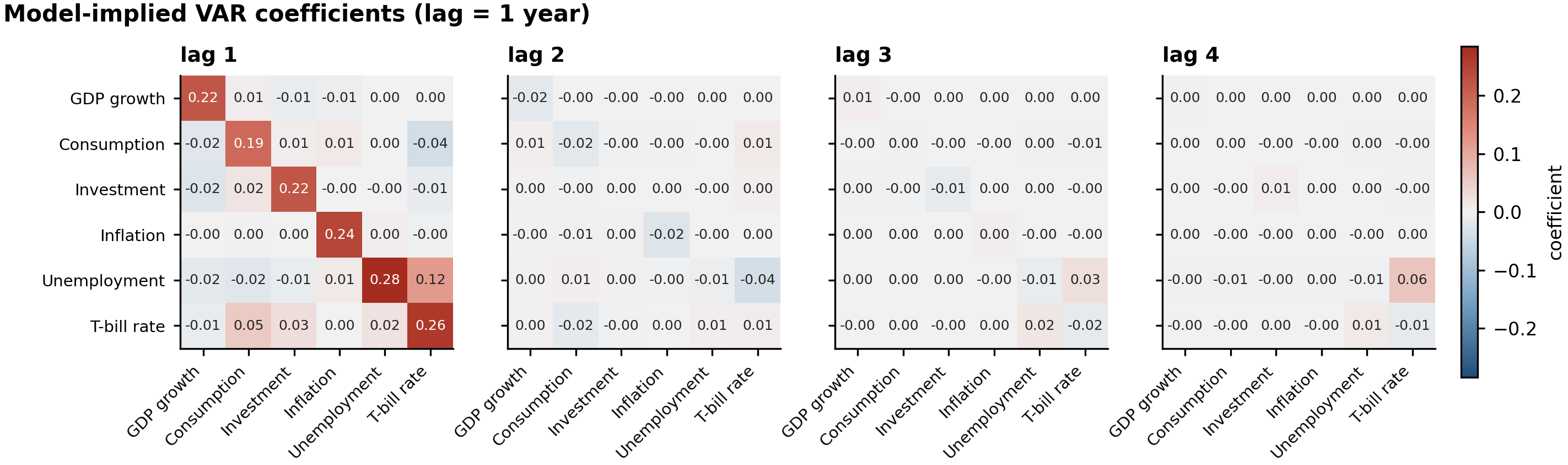
US quarterly macro: the lag matrices read straight out of the fitted network —
strong own-lag effects at one year, unemployment loading on the T-bill rate,
nothing left by lag 3. Produced by examples/02 in two minutes on a CPU.
These are the numbers this code actually produces on a laptop CPU, not numbers copied from the paper. Reproduce them with the commands in §11.
US quarterly macro, 6 series, 4-quarter horizon (examples/02, 60 epochs,
test = last 20 % of 1959Q2–2009Q3, standardised units):
| Model | MSE | MAE | RMSE |
|---|---|---|---|
| SaMoVAR | 0.4945 | 0.4835 | 0.7032 |
| AR(4) | 0.5161 | 0.4804 | 0.7184 |
| VAR(3), AIC | 0.6018 | 0.5350 | 0.7758 |
| Naive (RW) | 0.6059 | 0.5412 | 0.7784 |
| Ridge direct | 0.6330 | 0.5664 | 0.7956 |
Diebold–Mariano vs VAR(3): −1.33 (p = 0.19). Better point accuracy, not a significant difference on ~40 test origins — say so in your paper.
FRED-MD, 12 series, 12-month horizon, 1960–2019 (examples/03):
SaMoVAR 1.189 MSE vs VAR(4) 1.139 and AR(8) 1.149 — competitive, not dominant,
on 720 monthly observations. Widen the panel to 40 series and the classical VAR
collapses (MSE 2.65, worse than a random walk) while SaMoVAR degrades gracefully
to 1.095: the parameter count of the network does not grow with $C$, a VAR's
grows with $C^2p$.
Architectures on simulated VAR(3) data (examples/05, identical
tokenisation, loss and optimiser): at 8 epochs SaMoVAR 0.6766 < FixedVAR 0.6811
< LinTrans 0.6863, the paper's ordering; at 30 epochs all three sit within
0.004 MSE of each other (0.6316 / 0.6276 / 0.6311). A toy linear VAR does
not separate these architectures — the paper's separation comes from large real
benchmarks. Do not quote the short-budget ordering as evidence, and run the
ablations at --epochs 100 before reading anything into them.
Coefficient recovery on a known DGP (examples/04, VAR(2), 6000
observations): correlation between the recovered lag matrices and the truth
0.979, maximum absolute error 0.086.
| $A_1$ true | $A_1$ recovered | $A_2$ true | $A_2$ recovered | |
|---|---|---|---|---|
| y1←y1 | 0.60 | 0.648 | 0.15 | 0.150 |
| y1←y2 | 0.20 | 0.114 | −0.25 | −0.169 |
| y2←y1 | −0.10 | −0.046 | 0.30 | 0.225 |
| y2←y2 | 0.55 | 0.579 | 0.10 | 0.103 |
Forecast accuracy on that simulation: SaMoVAR 0.526 vs a correctly specified VAR(2) 0.481. On linear data generated by a VAR, a VAR wins — as it should. The gains this architecture is designed for appear with more observations, more series, and non-linear dynamics; the interpretation machinery is worth having either way.
11. Worked examples
| Script | What it demonstrates | Runtime (CPU) |
|---|---|---|
examples/01_quickstart.py |
fit → forecast → evaluate → benchmark → save/load on a simulated VAR(3) | ~1 min |
examples/02_us_macro_var.py |
full applied workflow on US quarterly macro data: descriptives + ADF, accuracy table, DM tests, IRFs vs a classical VAR, coefficient heatmaps | ~2 min |
examples/03_fred_md_benchmark.py |
12-variable FRED-MD monthly panel, 12-month horizon, full benchmark with per-series tables | ~5 min |
examples/04_interpretability.py |
coefficient recovery against a known DGP, influence paths, attention maps, time-varying coefficients | ~3 min |
examples/05_ablation_and_architectures.py |
SaMoVAR vs LinTrans vs FixedVAR, plus 11 component ablations | ~15 min |
python examples/01_quickstart.py --epochs 40
python examples/02_us_macro_var.py --epochs 150
python examples/03_fred_md_benchmark.py --epochs 120 --end 2019-12-01
python examples/04_interpretability.py --epochs 60
python examples/05_ablation_and_architectures.py --epochs 60
All outputs land in assets/.
12. Reproducing the paper's design choices
Defaults follow the paper: $d = 32\lfloor\sqrt{C}\rfloor$, head dimension 16, $l=3$, dropout 0.1, AdamW $(0.9, 0.95)$ with weight decay 0.1, one-cycle schedule with 5 % warm-up from lr/10, gradient clipping at 1.0, early stopping with patience 12.
Switches that reproduce specific rows of the paper's tables:
SaMoVAR(..., use_key_projection=True)      # Table 2  "w/ W_k"
SaMoVAR(..., structural_matrix="none")     # Table 2  "w/o D^-1"
SaMoVAR(..., qv_norm=False)                # Table 2  "w/o QV Norm"
SaMoVAR(..., n_heads=8)                    # Table 5  head-count ablation
SaMoVAR(..., n_layers=1)                   # Table 6  depth ablation
SaMoVAR(..., exogenous=False)              # univariate AR tokenisation
SaMoVAR(..., predictor="fixed")            # the FixedVAR control model
build_network(cfg, "lintrans")             # the LinTrans control model
The three places where the released code and the paper text disagree are resolved in favour of the code, since that is what produced the published numbers. To switch to the paper's equations instead:
SaMoVAR(..., structural_matrix="inverse",  # paper: D^-1; code multiplies by D
        shortcut_in_structural=True,       # paper: identity inside D
        normalization="revin")             # paper A.4: mean and std of the whole window
Where the paper, the released code and this implementation differ — including the three training bugs fixed here (gradient accumulation, clipping of scaled gradients, GradScaler under bf16) — is documented line by line in docs/THEORY.md.
13. Troubleshooting
"need at least input_length + horizon + 2 observations" — your sample is too short. Reduce input_length, or use VARForecaster from samovar.baselines.
Validation loss flat at ≈ 1.0 and forecasts near zero — the model is under-trained. Output weights start at std 0.02, so predictions begin near zero and must grow. Raise epochs, raise lr to 1e-3, or lower batch_size (fewer windows ⇒ fewer optimiser steps per epoch). Check model.history.to_frame() — if train_loss is still falling when training stops, it stopped too early.
A classical VAR beats SaMoVAR — on a short, linear, low-dimensional sample it should, and the library says so honestly. Neural gains appear with more observations, more series, and non-linear dynamics. Report both; the DM test tells you whether the gap is significant.
Out of memory on a wide panel — lower batch_size, raise accumulation_steps, lower d_model.
var_coefficients is slow or memory hungry — the exact recursion is $O(T^3 H d)$ in the intermediate step. Restrict channels (interpret.mixture_weights(..., series=[0,1])), reduce chunk, or use a larger horizon (fewer tokens).
Non-reproducible results — set seed=, and note that GPU non-determinism in cumsum reductions can still produce small differences run to run.
14. Citation and license
This library is an independent implementation. Please cite the original paper for the method:
@inproceedings{lu2025samovar,
  title     = {Linear Transformers as {VAR} Models: Aligning Autoregressive
               Attention Mechanisms with Autoregressive Forecasting},
  author    = {Lu, Jiecheng and Yang, Shihao},
  booktitle = {Proceedings of the 42nd International Conference on Machine Learning},
  series    = {PMLR},
  volume    = {267},
  year      = {2025},
  note      = {arXiv:2502.07244}
}
and, if the software itself was useful:
@software{roudane2026samovar,
  author  = {Roudane, Merwan},
  title   = {{SaMoVAR}: Structural Aligned Mixture of {VAR} for multivariate
             time series forecasting in {P}ython},
  year    = {2026},
  url     = {https://github.com/merwanroudane/SaMoVAR}
}
Released under the MIT License (see LICENSE). The reference implementation by Jiecheng Lu is also MIT-licensed; this package is a re-implementation written against the paper, with the architectural equations, ablation switches and training loop re-derived and documented.
Data sources used by the examples: statsmodels bundled datasets (BSD-3), and FRED-MD, downloaded on demand from the Federal Reserve Bank of St. Louis (McCracken & Ng, 2016) — no data files are redistributed with this repository.
1 maintainer

Metadata
1 maintainer
Release files for samovar-var 0.1.0
For a detailed explanation of source distributions (sdists) and built distributions (wheels), please see the package formats documentation.
Source distribution (sdist)
| File | Size | Uploaded | Provenance | |
|---|---|---|---|---|
| samovar_var-0.1.0.tar.gz | 100.6 kB | Without provenance | Details |
Built distribution (wheel)
| File | Interpreter | ABI | Platform | Reset |
|---|---|---|---|---|
| samovar_var-0.1.0-py3-none-any.whl | Python 3 | none | any | Details |
Total release size: 177.7 kB
Release files / samovar_var-0.1.0.tar.gz
| Download URL | samovar_var-0.1.0.tar.gz |
|---|---|
| Size | 100.6 kB |
| Tags | Source |
|
SHA-256 checksum How to use checksums |
3d1153c1a3b05c5d4550a218cf16205d6656e5fb245ffab157e40130b9b6fc23
|
|
BLAKE2b-256 checksum How to use checksums |
2929aade135e73f3fc5f67de9f96c5f7c7bbe70d7eb11a7ad8ec6cc0f78006ee
|
| Upload date | |
|
Uploaded using Trusted Publishing? What is trusted publishing? |
No |
| Uploaded via |
twine/7.0.0 CPython/3.11.0
|
Release files / samovar_var-0.1.0-py3-none-any.whl
| Download URL | samovar_var-0.1.0-py3-none-any.whl |
|---|---|
| Size | 77.1 kB |
| Tags | Python 3 |
|
SHA-256 checksum How to use checksums |
a82590df453109c2af9052d87d57475f272fd507cdde60229287a025566e4ed0
|
|
BLAKE2b-256 checksum How to use checksums |
f549f35ca1ff19ab0339dbbd9c0762aa5d89c2112110d073ec713838967a6472
|
| Upload date | |
|
Uploaded using Trusted Publishing? What is trusted publishing? |
No |
| Uploaded via |
twine/7.0.0 CPython/3.11.0
|
Security for samovar-var 0.1.0
Provenance
Provenance describes where a file came from. On PyPI, provenance is shared via attestations, which provide a verifiable record of the build or publishing details. View details, limitations and caveats.
No provenance found
None of the files in this release were uploaded with provenance metadata.
A note on package security
PyPI is a repository for distributing packages, not a service for auditing them. While third-party security researchers and our staff do their best to detect and remove malicious packages, PyPI cannot guarantee the quality, security or suitability of any given package.
To learn more about protecting yourself from malicious actors, visit our package security documentation.













