Scattertext extensions and iteroperabilties which require using code with viral licenses like GPL-*.

Project description
ScattertextVL
This is an extension to Scattertext interfacing with viral licensed code and data.
This package includes:
- wrappers for English USAS patterns (Piao et al. 2016) adapted from https://github.com/UCREL/Multilingual-USAS,
- wrappers around Biber register features, incorporating code from https://github.com/mshakirDr/MFTE (Le Foll and Shaki, 2023).
- wrappers around arguing features (Somoasundaran et al.) (2007).
Visualizing the UCREL Semantic Analysis System
The UCREL Semantic Analysis System (or USAS) (Piao et al., 2015) uses a set of lexico syntactic patterns to assign word-part-of-speech pairs and multi-word lexico-syntactic patterns to a hierarchy of semantic tags. Note that the use of this feature invokes the "Attribution-NonCommercial-ShareAlike 4.0 International" (CC BY-NC-SA 4.0) License.
474 semantic tags, arranged hierarchically, are tagged using the patterns. See the USAS Guide for an overview of the tag schema. The categories are organized into four tiers and are coded by an initial letter followed by three arabic numerals. I refer to tier 0, referring to most general tags containing no arabic numeral tier numbers, such as "A" ("General & Abstract Terms") or "B" ("The Body & the Individual"), to 3, the most specific tag, containing three arabic numerals-- for example, "A1.5.2" ("Usefulness"). Note that tiers 2 and 3 include tags from tiers 1 and 2 which do not contain any more specific categories.
By tier, the qualifying tag counts are:
| Tier | Count |
|---|---|
| 0 | 21 |
| 1 | 199 |
| 2 | 419 |
| 3 | 474 |
The USAS tagger produces an OffsetCorpus, which stores character offsets of USAS semantic tags so that, when a
tag is clicked in the Scattertext interface, the surface forms of each tag's patterns will appear in contexts.
Under the hood, the English USAS data is stored in 'scattertext/data/enusaspats.json.gz' as spaCy
EntityRuler patterns. The semantic tag ids are cross-referenced to the tag names present in
'scattertext/data/en_usas_subcategories.tsv.gz'. I have made some corrections to the patterns file (originally from
the [Multilingual-USAS Github repo]).
A spaCy model, which needs to include POS tagging, is passed to the USASOffsetGetter. Using a larger model will
likely result in better performance and definitely take longer to execute.
We plot tier 1 semantic tags on the political Convention corpus, with the x-axis representing the tag frequency dense rank and the y-axis the Hedge's $g$ effect size.
import scattertext as st
import scattertextvl as stvl
import spacy

nlp = spacy.blank('en')
nlp.add_pipe('sentencizer')

convention_df = st.SampleCorpora.ConventionData2012.get_data().assign(
    Party=lambda df: df.party.apply(lambda x: {'democrat': 'Dem', 'republican': 'GOP'}[x]),
    Parse=lambda df: df.text.progress_apply(nlp)
)

usas_offset_getter = stvl.USASOffsetGetter(
    tier=1,
    nlp=spacy.load('en_core_web_sm', disable=['ner'])
)

corpus = st.OffsetCorpusFactory(
    convention_df,
    category_col='Party',
    parsed_col='Parse',
    feat_and_offset_getter=usas_offset_getter
).build(show_progress=True)

score_df = st.CohensD(
    corpus
).use_metadata().set_categories(
    category_name='Dem'
).get_scosre_df(
)

plot_df = score_df.rename(
    columns={'hedges_g': 'HedgesG', 'hedges_g_p': 'HedgesGPval'}
).assign(
    Frequency=lambda df: df.count1 + df.count2,
    X=lambda df: df.Frequency,
    Y=lambda df: df.HedgesG,
    Xpos=lambda df: st.Scalers.dense_rank(df.X),
    Ypos=lambda df: st.Scalers.scale_center_zero_abs(df.Y),
    ColorScore=lambda df: df.Ypos,
)

html = st.dataframe_scattertext(
    corpus,
    plot_df=plot_df,
    category='Dem',
    category_name='Democratic',
    not_category_name='Republican',
    width_in_pixels=1000,
    suppress_text_column='Display',
    metadata=lambda c: c.get_df()['speaker'],
    use_non_text_features=True,
    ignore_categories=False,
    use_offsets=True,
    unified_context=False,
    color_score_column='ColorScore',
    left_list_column='ColorScore',
    y_label='Hedges G',
    x_label='Frequency Ranks',
    y_axis_labels=[f'More Dem: g={plot_df.HedgesG.max():.3f}', '0', f'More Rep: g={-plot_df.HedgesG.max():.3f}'],
    tooltip_columns=['Frequency', 'HedgesG'],
    term_description_columns=['Frequency', 'HedgesG', 'HedgesGPval'],
    header_names={'upper': 'Top Democratic', 'lower': 'Top Republican'},
    term_word_in_term_description='Semantic Tag',
    horizontal_line_y_position=0
)
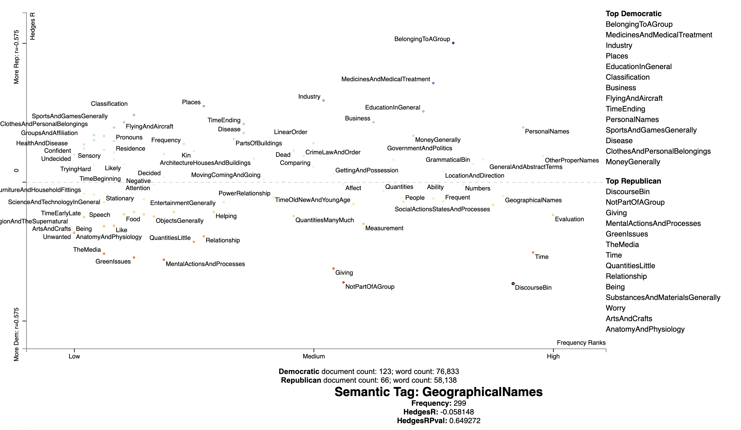
Clicking on a USAS tag can show us which phrases are recognized as surface forms. This also serves as a way of debugging and improving patterns.
We can plot the full USAS tag set by not including a tier parameter:
usas_offset_getter = stvl.USASOffsetGetter(
    tier=1,
    nlp=spacy.load('en_core_web_sm', disable=['ner'])
)
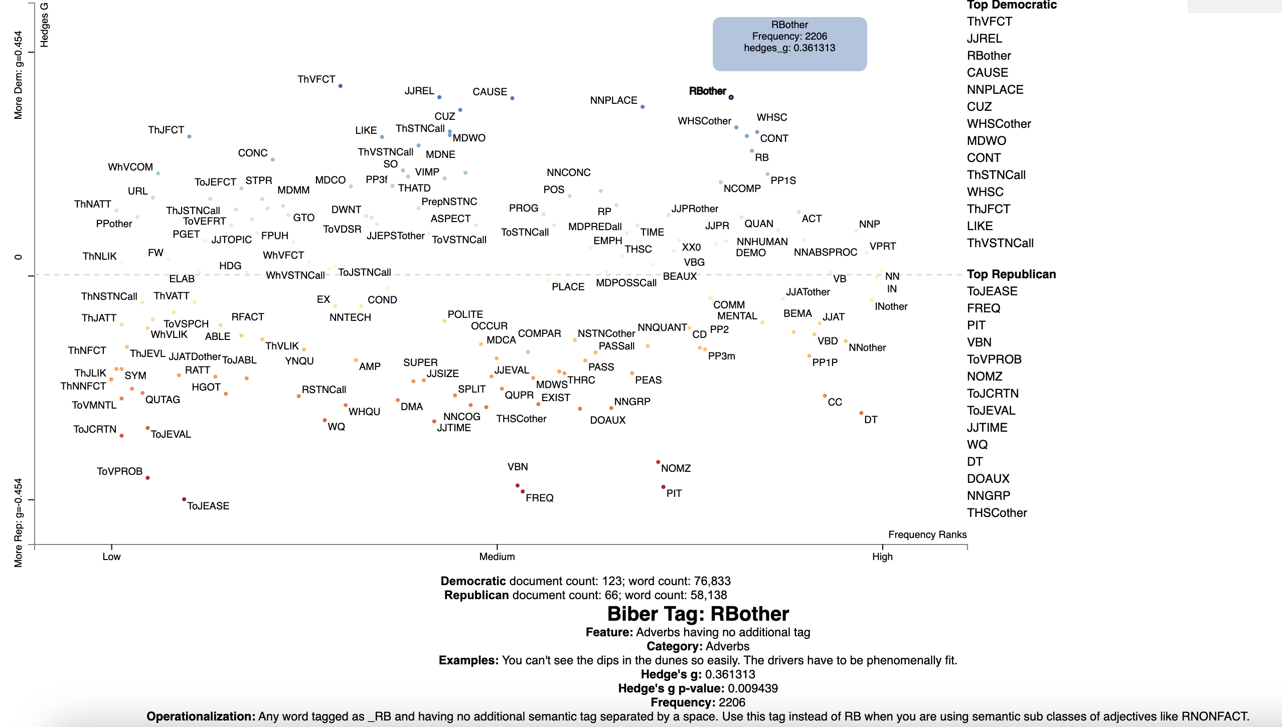
Visualizing Biber Register Features
ScattertextVL contains a modified version of MTFE (Le Foll and Shaki, 2023) which provides a way of labeling the Biber tagset.
One can preview the feature set here using:
stvl.get_biber_feature_df().head()
Note that the first column contains the feature codes, used in the visualization, for the Biber set.
| Category | Feature | Examples | Operationalization | NormalizationUnit | |
|---|---|---|---|---|---|
| Words | General text properties | Total number of words | It's a shame that you'd have to pay to get that quality. (= 14) | The number of tokens as tokenised by the Stanford Tagger, but excluding punctuation marks, brackets, symbols, genitive ‘s (POS), and filled pauses and interjections (FPUH). Contractions are treated as separate words, i.e., it's is tokenised as it and 's. Note that this variable is only used to normalise the frequencies of other linguistic features. | |
| AWL | General text properties | Average word length | It's a shame that you'd have to pay to get that quality. (42/12 = 3.50) | Total number of characters in a text divided by the number of words in that same text (as operationalised in the Words variable above, hence excluding filled pauses and interjections, cf. FPUH). | Words |
| TTR | General text properties | Lexical diversity | It's a shame that you'd have to pay to get that quality. (12/14 = 0.85) | Following Biber (1988), this feature is a type-token ratio measured on the basis of, by default, the first 400 words of each text only. It is thus the number of unique word forms within the first 400 words of each text divided by 400. This number of words can be adjusted in the command used to run the script (see instructions at the top of the MFTE script). | Words (by default first 400) |
| LDE | General text properties | Lexical density | It's a shame that you'd have to pay to get that quality. (3/14 = 0.21) | For this feature, tokens which are not on the list of the 352 function words from the {qdapDictionaries} R package, nor individual letters, or any of the fillers listed in FPUH are identified as content words. Lexical density is calculated as the ratio of these content words to the total number of words in a text. | Words |
| FV | General text properties | Finite verbs | He discovered that the method involved imbiding copious amounts of tea. Ants can survive by joining together to morph into living rafts. Always wanted to experience the winter wonderland that Queen Elsa created? | This feature is not directly listed in the MFTE output tables; however, it is used as a normalisation basis for many other linguistics features (see Normalisation column). It is calculated by tallying the number of occurrences of the following features: VPRT, VBD, VIMP, MDCA, MDCO, MDMM, MDNE, MDWO and MDWS. |
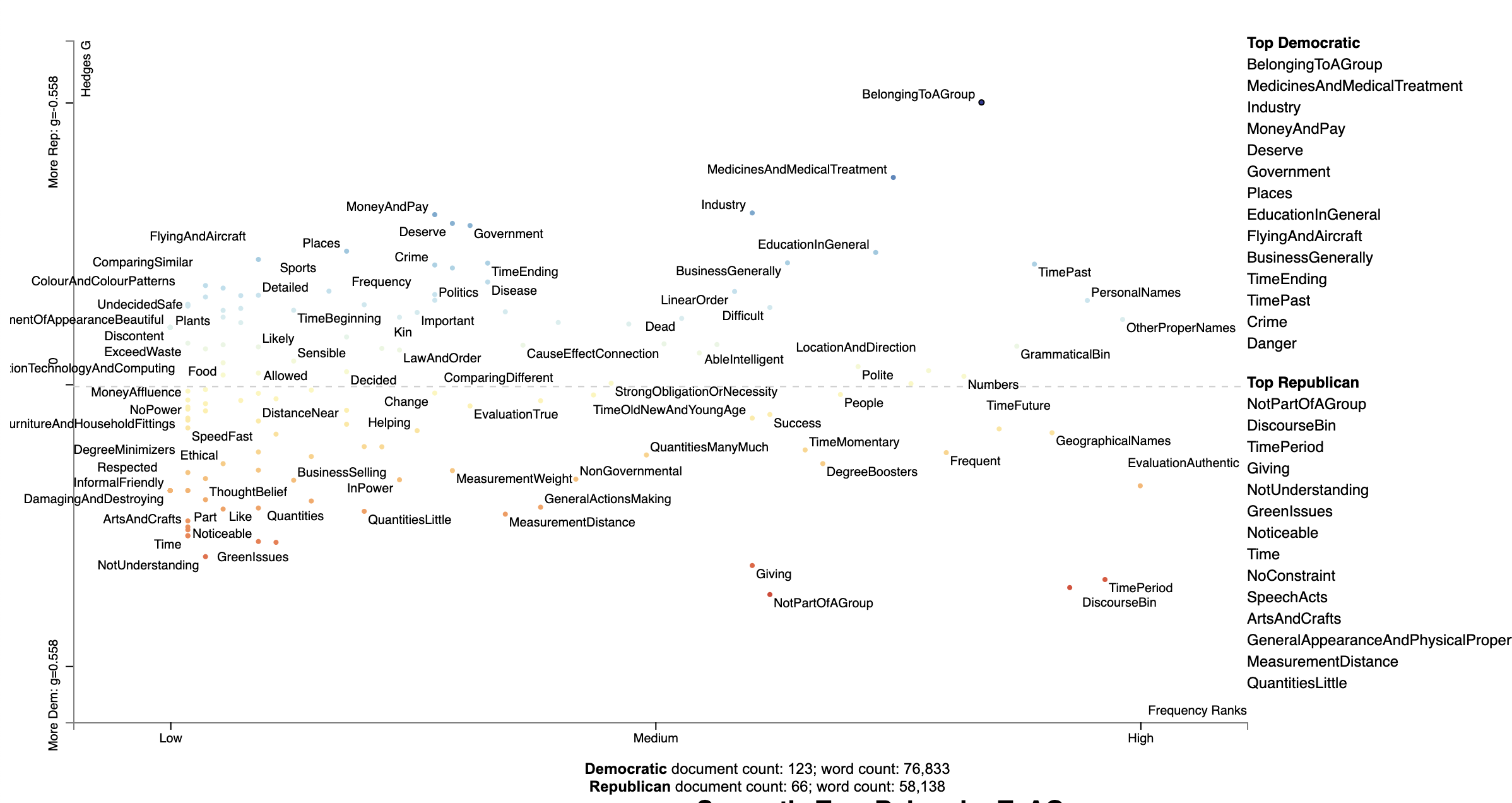
We can visualize the Biber feature set using the following code to set up the plot_df data frame, using Hedge's $g$ as
the distinctivenes scoring function. Note that we merge in the feature description data frame,
stvl.get_biber_feature_df(), before visualizing.
biber_corpus = st.OffsetCorpusFactory(
    convention_df,
    category_col='Party',
    parsed_col='Parse',
    feat_and_offset_getter=stvl.BiberOffsetGetter()
).build(show_progress=True)

biber_stat_df = st.HedgesG(
    biber_corpus
).use_metadata().set_categories(
    category_name='Dem'
).get_score_df(
).assign(
    Frequency=lambda df: df.count1 + df.count2,
    X=lambda df: df.Frequency,
    Y=lambda df: df.hedges_g,
    Xpos=lambda df: st.Scalers.dense_rank(df.X),
    Ypos=lambda df: st.Scalers.scale_center_zero_abs(df.Y),
    ColorScore=lambda df: df.Ypos,
)

plot_df = pd.merge(
    biber_stat_df,
    stvl.get_biber_feature_df(),
    left_index=True,
    right_index=True
).reset_index().rename(columns={'index': 'term'}).set_index('term')
Finally, we produce the interactive visualization using:
st.dataframe_scattertext(
    biber_corpus,
    plot_df=plot_df,
    category='Dem',
    category_name='Democratic',
    not_category_name='Republican',
    width_in_pixels=1000,
    suppress_text_column='Display',
    metadata=lambda c: c.get_df()['speaker'],
    use_non_text_features=True,
    ignore_categories=False,
    use_offsets=True,
    unified_context=False,
    horizontal_line_y_position=0,
    color_score_column='ColorScore',
    left_list_column='ColorScore',
    y_label='Hedges G',
    x_label='Frequency Ranks',
    y_axis_labels=[f'More Dem: g=-{plot_df.hedges_g.abs().max():.3f}',
                   '0',
                   f'More Rep: g={plot_df.hedges_g.abs().max():.3f}'],
    tooltip_columns=['Frequency', 'hedges_g'],
    term_description_columns=['Feature', 'Category', 'Examples',
                              'hedges_g', 'hedges_g_p', 'Frequency', 'Operationalization'],
    term_description_column_names={'hedges_g': "Hedge's g",
                                   'hedges_g_p': "Hedge's g p-value"},
    header_names={'upper': 'Top Democratic', 'lower': 'Top Republican'},
    term_word_in_term_description='Biber Tag',
)
Visualizing Arglex Discourse Arguing Features
Somasundaran et al. (2007) compiled a set of regular expressions matching language describing different types of arguing for or against a point in meeting corpora. These appear to yield interesting results in the political convention example.
References
Le Foll, E., & Shakir, M. 2023. MFTE Python (Version 1.0) https://github.com/mshakirDr/MFTE
Le Foll, Elen. 2021. A New Tagger for the Multi-Dimensional Analysis of Register Variation in English. Osnabrück University: Institute of Cognitive Science Unpublished M.Sc. thesis.
Biber, Douglas. 1984. A model of textual relations within the written and spoken modes. University of Southern California. Unpublished PhD thesis.
Biber, Douglas. 1988. Variation across speech and writing. Cambridge: Cambridge University Press.
Biber, Douglas. 1995. Dimensions of Register Variation. Cambridge, UK: Cambridge University Press.
Biber, D. 2006. University language: A corpus-based study of spoken and written registers. Benjamins.
Biber, D., Johansson, S., Leech, G., Conrad, S., & Finegan, E. 1999. Longman Grammar of Spoken and Written English. Longman Publications Group.
Conrad, Susan & Douglas Biber (eds.) 2013. Variation in English: Multi-Dimensional Studies (Studies in Language and Linguistics). New York: Routledge.s
Scott Piao, Paul Rayson, Dawn Archer, Francesca Bianchi, Carmen Dayrell, Mahmoud El-Haj, Ricardo-María Jiménez, Dawn Knight, Michal Křen, Laura Löfberg, Rao Muhammad Adeel Nawab, Jawad Shafi, Phoey Lee Teh, and Olga Mudraya. 2016. Lexical Coverage Evaluation of Large-scale Multilingual Semantic Lexicons for Twelve Languages. In Proceedings of the Tenth International Conference on Language Resources and Evaluation (LREC'16), pages 2614–2619, Portorož, Slovenia. European Language Resources Association (ELRA).
Swapna Somasundaran, Josef Ruppenhofer and Janyce Wiebe (2007) Detecting Arguing and Sentiment in Meetings, SIGdial Workshop on Discourse and Dialogue, Antwerp, Belgium, September 2007 (SIGdial Workshop 2007).
Release history Release notifications | RSS feed

Download files
Download the file for your platform. If you're not sure which to choose, learn more about installing packages.
Source Distribution
File details
Details for the file scattertextvl-0.1.0.tar.gz.
File metadata
- Download URL: scattertextvl-0.1.0.tar.gz
- Upload date:
- Size: 3.8 MB
- Tags: Source
- Uploaded using Trusted Publishing? No
- Uploaded via: twine/5.0.0 CPython/3.11.0
File hashes
| Algorithm | Hash digest | |
|---|---|---|
| SHA256 |
0c11c2bb1344d765c10da832a627b3192df4ebe205b139889fecca0e2f97bafc
|
|
| MD5 |
e6f6f1101488232ec56ecf347c08b305
|
|
| BLAKE2b-256 |
aefada0a842c78bc6150f6a9fd5a387960f789c28fe6394665da34d3da52f2ff
|


