
scCont


scCont is an unsupervised contrastive deep learning model that extracts interpretable latent features from single-cell RNA data.
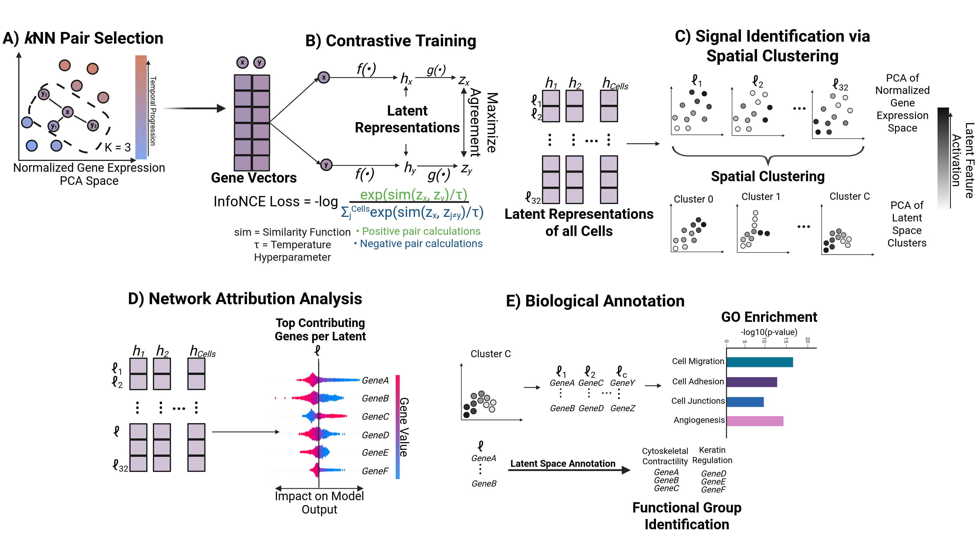
Contrastive learning is typically used to find similarities between actual and perturbed data, but we modify the typical contrastive learning framework to use the framework to learn local neighborhood functional group information in scRNA data. scCont achieves this through five steps: 1) _k_NN Pair Selection, 2) Contrastive Training, 3) Signal Identification via Spatial Clustering, 4) Network Attribution Analysis, 5) Biological Annotation. Figure 1 visualizes these steps.
Installation
pip install sccont
One install covers every stage, including preprocessing (Scrublet) and GO enrichment (g:Profiler).
Requires Python 3.10+. pip installs a CPU build of PyTorch by default; for GPU training install
torch first following https://pytorch.org/get-started/locally/, then install sccont.
To work from a source checkout instead:
git clone https://github.com/nramani611/scCont.git
cd scCont
pip install -e ".[dev]"
pytest
Quickstart
scCont works on an AnnData object (cells x genes). Put any
per-cell labels you have (timepoint, condition, batch, cluster, ...) in adata.obs; they are
carried through every step and used for interpretation and plotting. Training itself is
unsupervised and never reads them. Results are written back onto the same object:
| Where | What |
|---|---|
adata.obsm["X_sccont"] |
latent features, cells x 32 |
adata.obsm["X_sccont_pca"] |
PCA of the latent space |
adata.varm["sccont_shap_mean_abs"] |
mean |SHAP| per gene and latent feature |
adata.uns["sccont"] |
latent key, latent dimension, spatial cluster labels |
import sccont

sccont.set_seeds(42)                                   # all paper results use seed 42

# Any AnnData of raw counts works. The repo's genes x cells tables convert like this:
counts = sccont.load_expression_matrix("MCF10A_TGFB1/GSE200981_scRNAseq_processed.tsv")
adata = sccont.to_anndata(counts, timepoint=sccont.timepoints_from_columns(counts.columns))
# adata.obs["condition"] = ...                         # add any other labels you have

# Normalise (skip if adata.X is already normalised); obs labels are preserved
adata = sccont.preprocess(adata)                       # QC, Scrublet, log-norm, 3000 HVGs, regress, scale

# A) kNN positive pairs
pairs = sccont.get_knn_pairs(adata, k=3)

# B) Contrastive training + embedding (latents -> adata.obsm["X_sccont"])
encoder, projector, losses = sccont.train_contrastive(adata, pairs, latent_dim=32, epochs=20000)
sccont.embed(encoder, adata)
sccont.save_encoder(encoder, "encoder.pth")

# C) Spatial clustering of latent features
sccont.elbow_plot_for_clusters(adata, max_k=12)        # pick n_groups from the elbow
groups, _ = sccont.group_spatially_similar_latents(adata, n_groups=3)

# D) Network attribution (SHAP): cells x genes x latents; summary -> adata.varm
shap_values = sccont.compute_shap_values(encoder, adata)
gene_names = list(adata.var_names)
top_genes = sccont.select_top_genes_by_zscore(shap_values, gene_names, latent_feature_index=7)

# E) GO enrichment per spatial cluster (network call to g:Profiler)
go_results = sccont.enrich_latent_clusters(shap_values, gene_names, groups)
sccont.write_go_results_excel(go_results, "GO_Enrichment_Results.xlsx")

# Latent features as an AnnData of their own (obs labels copied) for plotting / scanpy tools
adata_latent = sccont.latent_anndata(adata)
Reusing a trained encoder shipped in this repository:
encoder = sccont.load_encoder("MCF7_TNF/encoder.pth", input_dim=adata.n_vars, latent_dim=32)
Arrays still work everywhere an AnnData is accepted (cells x genes), and the original
TemporalSingleCellDataset(genes_x_cells, timepoints) container is kept for backwards compatibility.
Every preprocessing step has its own switch, so you can turn off the ones that do not apply to your data. For example, simulated data with no mitochondrial or cell-cycle signal:
adata = sccont.preprocess(
    adata,
    remove_doublets=False,      # skip Scrublet
    max_pct_mito=None,          # no mitochondrial filter
    regress_mito=False,
    regress_cell_cycle=False,
)
The full list of switches (min_genes, max_genes, max_pct_mito, min_cells, remove_doublets,
normalize_total, log1p, n_top_genes, regress_mito, regress_counts, regress_cell_cycle,
scale) is documented in help(sccont.preprocess).
API overview
| Stage | Function | Purpose |
|---|---|---|
| — | set_seeds, get_device |
Reproducibility, device selection |
| — | load_expression_matrix, to_anndata, timepoints_from_columns |
Read the repo's genes x cells tables and build an AnnData with labels in obs |
| — | preprocess |
QC / normalise an AnnData (every step switchable), obs preserved |
| A | get_knn_pairs |
kNN positive pairs in PCA space (labels ignored) |
| B | Encoder, Projector, InfoNCELoss |
Network components |
| B | train_contrastive, embed, latent_anndata, save_encoder, load_encoder |
Train; write latents to adata.obsm; latent-features-as-variables view; persist weights |
| C | elbow_plot_for_clusters, group_spatially_similar_latents, latents_in_group |
Cluster latent features by spatial pattern (stored in adata.uns) |
| D | compute_shap_values, select_top_genes_by_zscore, top_genes_per_latent |
Gene -> latent attributions (summary in adata.varm) |
| E | enrich_latent_clusters, run_go_enrichment, write_go_results_excel, collect_enriched_genes |
GO enrichment |
| E | latent_report, gene_directions, annotate_latent, annotate_latents |
Per-latent driver report for any LLM; optional Claude-assisted functional groups (sccont[llm]) |
| — | pl.* |
Plotting from the stored results (see below) |
Every function has a docstring; help(sccont.preprocess) lists all QC parameters.
Plotting
sccont.pl draws from the results stored on the AnnData and colours by any obs column.
Every function accepts ax=, show= and save= and returns the matplotlib axes.
pl = sccont.pl
pl.training_loss(losses)
pl.latent_embedding(adata, color="timepoint")            # any obs column, or a latent index: color=7
pl.latent_grid(adata)                                     # every latent's activation, ordered by spatial group
pl.latent_distance_heatmap(adata)                         # the matrix behind the spatial grouping
pl.latent_by_label(adata, 7, "condition", kind="violin")
pl.latent_label_association(adata, "timepoint")          # which latents track a label (heatmap / correlations)
pl.top_genes(adata, latent=7, shap_values=shap_values)   # mean |SHAP| bars, coloured by direction
pl.go_enrichment(go_results)                              # dot plot per spatial cluster
Manuscript-style figures, generalised to any ordered label:
pl.group_trajectories(adata, groupby="timepoint", split_after="T2")           # Figure 2
pl.gene_set_shap_embedding(adata, shap_values, genes, latent=7)
pl.shap_beeswarm(adata, shap_values, latent=7)
pl.assign_branches(adata, shap_values, latent=7, genes=genes)                 # -> obs["sccont_branch"]
pl.functional_group_heatmap(adata, shap_values, functional_groups, group_to_latent,
                            groupby="timepoint", branch_key="sccont_branch")  # linear or bifurcating layout
pl.latent_trajectory(adata, shap_values, gene_sets, latents=[0, 5], groupby="timepoint")
Colour conventions: distinct labels use a fixed eight-colour palette, ordered labels and magnitudes a single blue ramp, and signed quantities (latent activation, z-scores, SHAP sums) a blue-grey-red scale centred on zero.
Optional: LLM-assisted functional-group annotation
Turning a latent feature's driver genes into named functional groups (pathways, processes, cell states) normally means a literature search. As a convenience, scCont can hand that step to a large language model. This is entirely optional; the core pipeline never calls an LLM.
Important: LLMs can hallucinate. A model may invent pathway memberships, misattribute a gene's function, or state a confident rationale with no support in the literature. Treat every proposed group as a hypothesis: check each gene's assignment against primary sources or curated databases (e.g. GO, Reactome, KEGG, UniProt) before using it in an analysis or publication. scCont only constrains the output to genes present in the report; it cannot verify the biology.
Option 1: build the description and paste it into the assistant of your choice.
report = sccont.latent_report(adata, shap_values, latent=7, go_results=go_results,
                              groupby="timepoint", invert=True)
print(report.to_prompt())      # positive/negative driver genes, label association, GO terms
report.to_frame()              # the same drivers as a table
Option 2: query Claude directly from Python.
pip install "sccont[llm]"
export ANTHROPIC_API_KEY=...   # or `ant auth login`
result = sccont.annotate_latents(adata, shap_values, latents=[0, 5, 6, 7],
                                 go_results=go_results, groupby="timepoint",
                                 invert_shap={7: True}, extra_context="MCF10A cells, TGF-beta1 time course")
result.functional_groups       # {name: [genes]}  – same format as functional_groups.json
result.group_to_latent         # {name: latent}   – same format as group_to_latent.json
result.table                   # group, latent, genes, direction, confidence, rationale – review this
result.save("my_dataset/")     # writes the JSON files (+ annotations.csv) for the notebook and pl.functional_group_heatmap
Each latent is one structured-output request to claude-opus-5 (a few cents per latent). Genes not
in the report are discarded, and every group carries a rationale and a confidence rating to guide
your review. Pass model= to use a different Claude model and client= to supply your own
configured anthropic.Anthropic client.
Tutorial notebook
scCont Pipeline.ipynb walks through the five stages on the MCF10A TGFB1 dataset using the
package API, then reproduces the latent-level analysis and manuscript figures (functional-group
heatmaps and multi-latent trajectory plots). Run it with the cont-learn kernel or any environment
where sccont and jupyter are installed.
Simulated data (SERGIO)
The simulation benchmark in the manuscript uses SERGIO
with explicit ground-truth gene programs. simulation/ contains the exact scripts and per-run
parameter files used to generate every simulated dataset, plus a normalisation step that matches
the real-data pipeline. See simulation/README.md for setup and the
command that reproduces each dataset.
Repository Structure & Data
There are 13 folders in this repository - one for each dataset benchmarked in the study. Due to GitHub file size limits, some of the .gz datasets are hosted externally. All full datasets used to train scCont are available via this Google Drive link.
The following files are available for all datasets:
.gzfile: The processed dataset used to train scCont.GO_Enrichment_Results.xlsx: GO enrichment results from each cluster (calculated post-Stage 3). Each sheet corresponds to a different spatial cluster.encoder.pth: The saved PyTorch weights of the encoder function after training (load withsccont.load_encoder).
Specific Dataset Annotations
The MCF10A_TGFB1 folder and all A549 dataset folders contain additional metadata used to generate manuscript figures:
functional_groups.json: Dictionary mapping functional group names to the specific genes involved.group_to_latent.json: Dictionary mapping functional group names to their source latent feature index.invert_shap.json: Dictionary mapping latent features to a boolean indicating if SHAP values were inverted to establish a positive correlation with experimental time.latent_to_bifurcation.json: Dictionary mapping latent features to a boolean indicating if it was identified as a bifurcating trajectory (Note: This analysis is specific to the MCF10A_TGFB1 dataset).
Other files:
src/sccont/– the installable package.tests/– pytest suite (runs on CPU in a few seconds).requirements.txt– the exact frozen environment used for the manuscript, kept for reproducibility. The package's own dependencies are declared inpyproject.toml.RELEASING.md– how releases are published to PyPI.
Contact
If you have any questions, encounter issues, or need help adapting scCont for your own data, please open an issue on this repository or contact the corresponding author, Neal Kewalramani, at nramani@bu.edu.
1 maintainer

Metadata
1 maintainer
Release files for sccont 0.1.0
For a detailed explanation of source distributions (sdists) and built distributions (wheels), please see the package formats documentation.
Source distribution (sdist)
| File | Size | Uploaded | |
|---|---|---|---|
| sccont-0.1.0.tar.gz | 57.8 kB | Details |
Built distribution (wheel)
| File | Interpreter | ABI | Platform | Reset |
|---|---|---|---|---|
| sccont-0.1.0-py3-none-any.whl | Python 3 | none | any | Details |
Total release size: 106.7 kB
Release files / sccont-0.1.0.tar.gz
| Download URL | sccont-0.1.0.tar.gz |
|---|---|
| Size | 57.8 kB |
| Tags | Source |
|
SHA-256 checksum How to use checksums |
853ef6da6db375fcb4fbd28fc76654e423f676d74061a0850c826a3adb7a0f9c
|
|
BLAKE2b-256 checksum How to use checksums |
4454a8f0f002ff6bffb603ca028e566ee259a66937f707c765a06f5c64e8f4c7
|
| Upload date | |
|
Uploaded using Trusted Publishing? What is trusted publishing? |
Yes |
| Uploaded via |
twine/7.0.0 CPython/3.13.14
|
Provenance
Provenance describes where a file came from. On PyPI, provenance is shared via attestations, which provide a verifiable record of the build or publishing details. View details, limitations and caveats.


PyPI Publish Attestation
PyPI verified that this artifact, at this checksum, originated from the publisher listed below.
Signed by GitHub Actions, verified by PyPI on Sep 23, 2026.
Transparency logRelease files / sccont-0.1.0-py3-none-any.whl
| Download URL | sccont-0.1.0-py3-none-any.whl |
|---|---|
| Size | 48.9 kB |
| Tags | Python 3 |
|
SHA-256 checksum How to use checksums |
7ce3a0d5c69c20f7695cd056d68f3217945223d89566036c752ad34c0988cfda
|
|
BLAKE2b-256 checksum How to use checksums |
edadb7bc89545e24b767c88ce047e0072430f97dc08fe96ee99666ad0d7c2f2f
|
| Upload date | |
|
Uploaded using Trusted Publishing? What is trusted publishing? |
Yes |
| Uploaded via |
twine/7.0.0 CPython/3.13.14
|
Provenance
Provenance describes where a file came from. On PyPI, provenance is shared via attestations, which provide a verifiable record of the build or publishing details. View details, limitations and caveats.
PyPI Publish Attestation
PyPI verified that this artifact, at this checksum, originated from the publisher listed below.
Signed by GitHub Actions, verified by PyPI on Sep 23, 2026.
Transparency log












