A comprehensive Python framework for seismic surface wave forward modeling and inversion.

Project description
SeisWave


SeisWave is a comprehensive Python framework for seismic surface wave forward modeling and dispersion inversion. By natively supporting Full $f-c$ (Frequency-Phase Velocity) Spectrum Inversion, it eliminates the need for manual, error-prone dispersion curve picking, making it highly robust to noise and seamlessly incorporating higher modes. It integrates native Python modeling algorithms alongside robust memory-bound Fortran extensions derived from Computer Programs in Seismology (CPS), offering researchers both flexibility and standard-compliant high-performance computations.
Features
- Forward Modeling: Generate synthetic seismograms and $f-c$ phase velocity dispersion images from 1D earth models.
- Dispersion Inversion (Full $f-c$ Spectrum Approach):
Instead of relying on manual, error-prone dispersion curve picking,
seiswavedirectly inverts the entire $f-c$ energy image. This preserves crucial amplitude variations, naturally incorporates higher modes without mathematical separation, and provides superior robustness against field data noise.- Differential Evolution (DE): Fast global optimization for quick Earth model approximations.
- MCMC Bayesian Inference: Comprehensive probabilistic inversion outputting Posterior distributions, credible intervals, and full acceptance-rejection & $\hat{R}$ diagnostics.
- CPS Fortran Integration: Bypasses slow I/O
subprocesscalls by binding Fortran routines (likesdisp96,sregn96,spulse96) directly to Python memory space usingf2py. - Interactive Web UI: A fully-featured modern Streamlit interface seamlessly bundled with the package, eliminating the need to write Python scripts for standard analysis workflows.
Installation
As this package automatically compiles high-performance Fortran extensions (f2py), you must have a Fortran compiler installed. The most reliable and cross-platform way to install seiswave is by using a conda environment.
Using Conda (Windows, macOS, & Linux)
First, create a fresh Python environment and install the required compiler tools (m2w64-toolchain for Windows, or gfortran for Unix):
Windows:
conda create -n seiswave python=3.11
conda activate seiswave
conda install conda-forge::gfortran_win-64 # Installs MinGW gfortran
pip install seiswave
macOS / Linux:
conda create -n seiswave python=3.11
conda activate seiswave
conda install -c conda-forge gfortran
pip install seiswave
Quick Launch
seiswave-web
(Note: If Streamlit prompts you for an email address upon the first launch, simply leave it blank and press Enter.)
Gallery
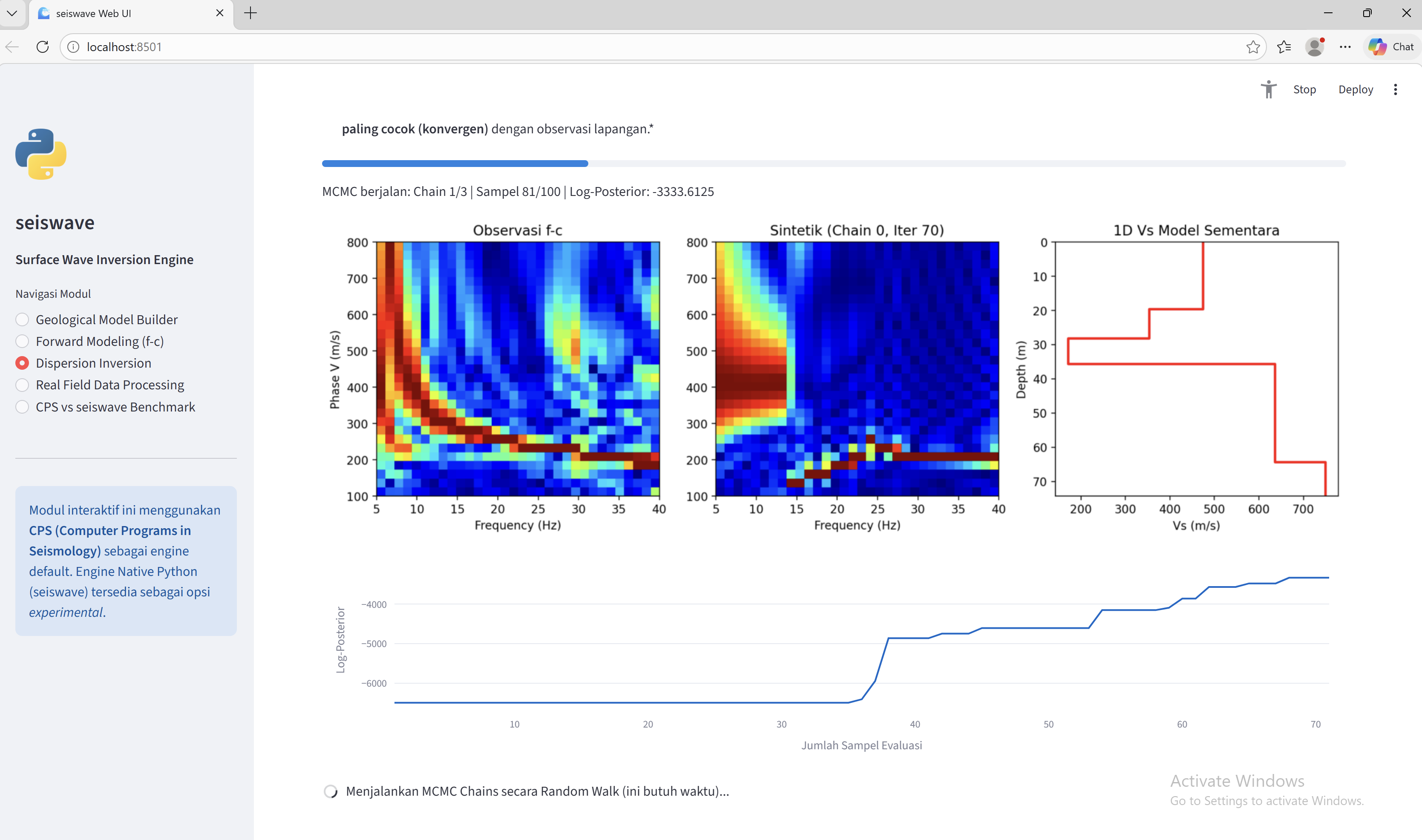
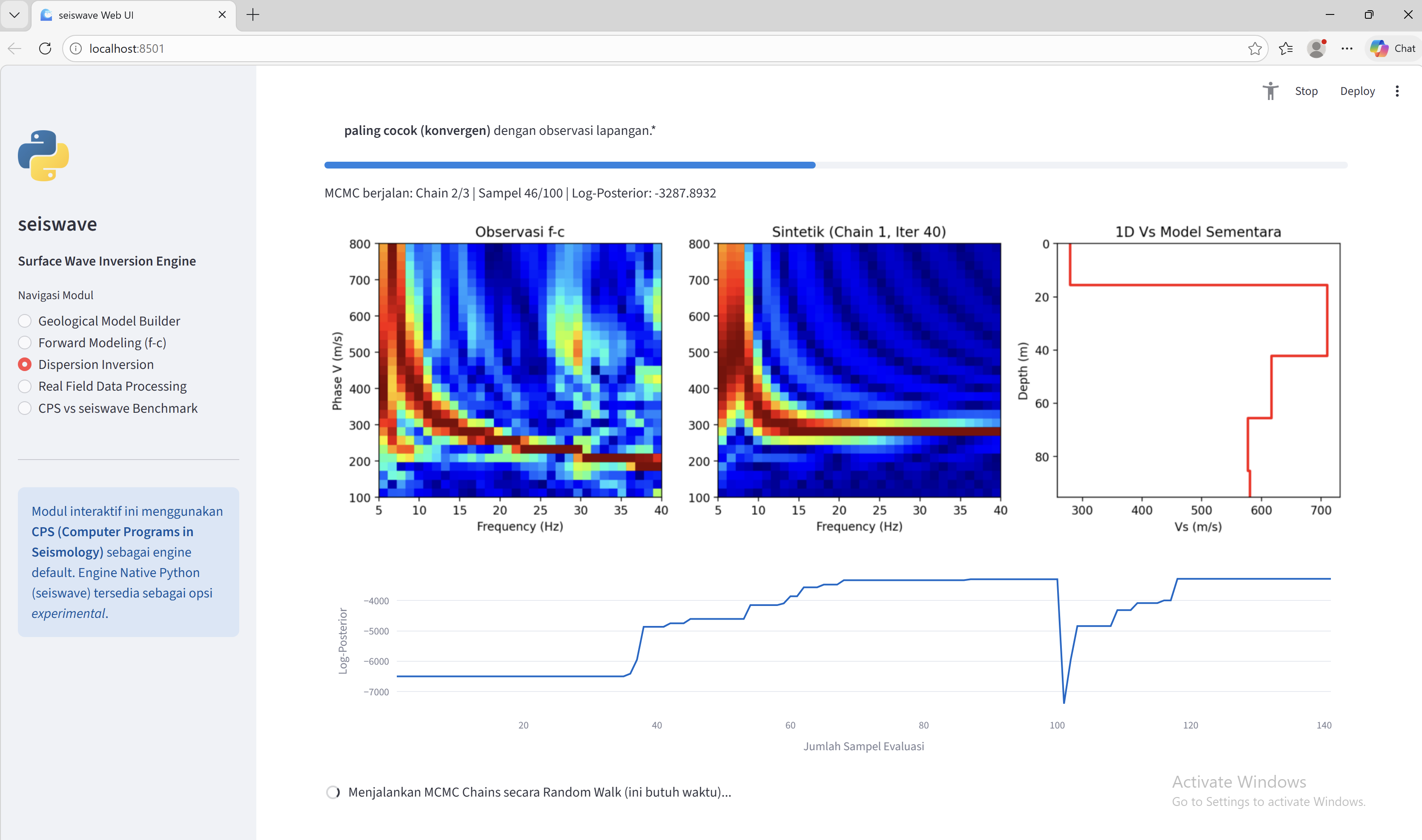
MCMC Inversion Process snapshots
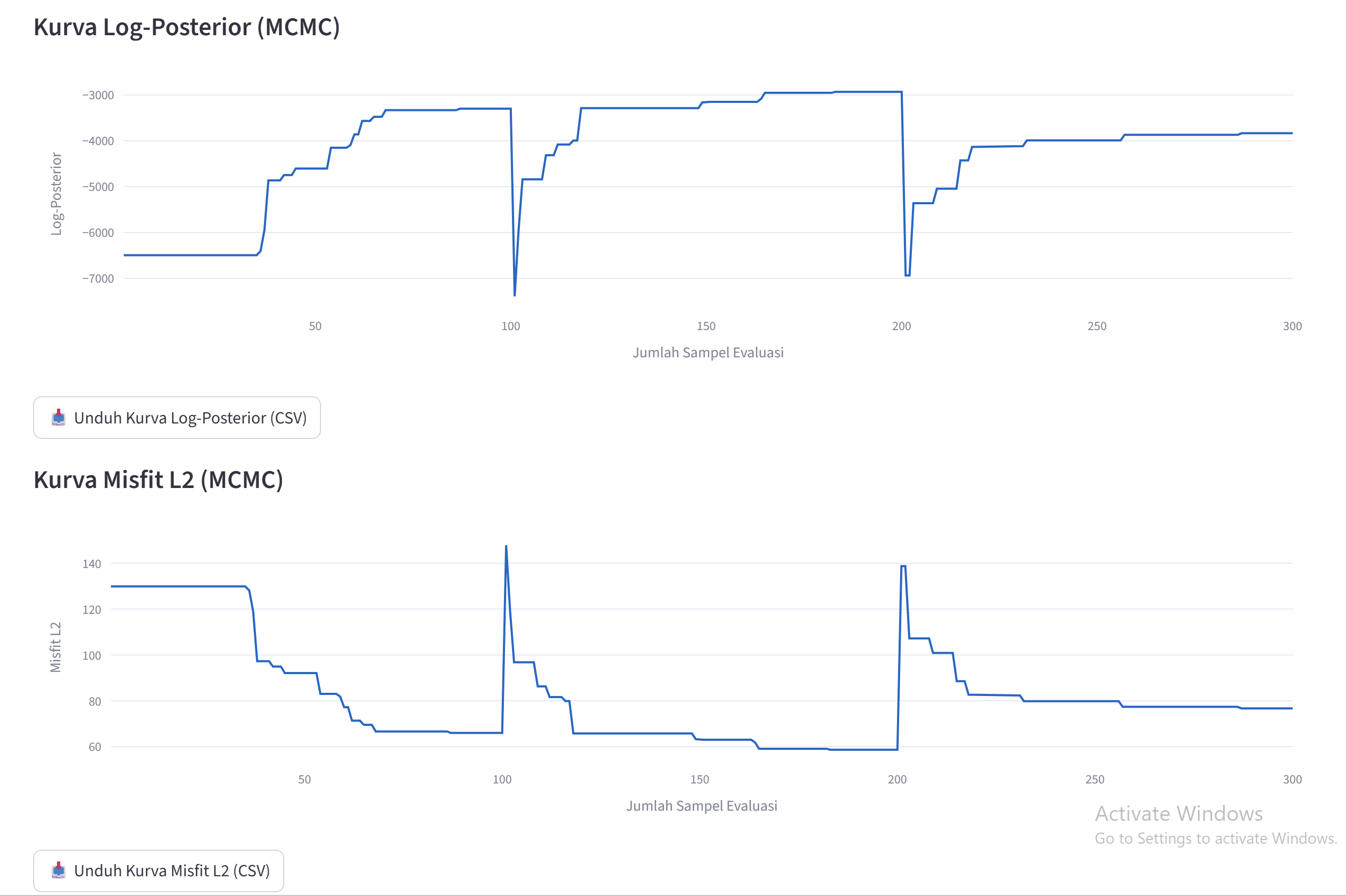
Statistical Diagnostics
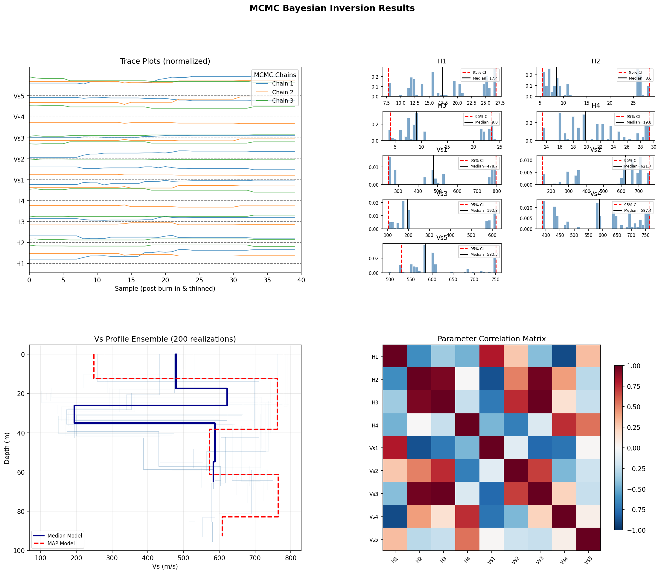
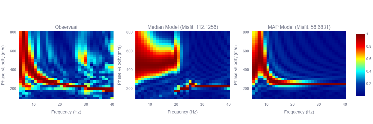
Result Comparisons
Methodological Details
1. Earth Model Parametrization
To reduce the non-uniqueness of the inversion problem, seiswave only requires the user to invert for Layer Thicknesses ($H$) and S-wave velocities ($V_s$). The other dependent parameters are automatically derived using Brocher's (2005) empirical relationships (note: $V_s$ and $V_p$ are in km/s for these formulas):
- P-wave velocity ($V_p$): $$V_p = 0.9409 + 2.0947 V_s - 0.8206 V_s^2 + 0.2683 V_s^3 - 0.0251 V_s^4$$
- Density ($\rho$): Computed from P-wave velocity ($V_p$) in g/cm³: $$\rho = 1.6612 V_p - 0.4721 V_p^2 + 0.0671 V_p^3 - 0.0043 V_p^4 + 0.000106 V_p^5$$
- Quality Factors ($Q_s, Q_p$): Estimated based on standard attenuation guidelines (with $V_s$ in m/s): $$Q_s = \frac{V_s}{10.0}, \quad Q_p = 2.0 \times Q_s$$
2. Inversion Workflow
2.1 Differential Evolution (DE) Global Optimization
DE is a stochastic population-based algorithm used for rapidly searching the global parameter space to find an optimal approximate 1D Earth model.
graph TD
    A[Observed Data: f-c Spectrum E_obs] --> B[Initialize Population: H & Vs Bounds]
    B --> C[Evaluate Initial Population L2 Misfit]
    C --> D[Begin DE Iteration]
    D --> E[Mutation: Create Donor Vectors]
    E --> F[Crossover: Generate Trial Vectors]
    F --> G[Forward Modeling: Synthetic f-c Spectrum]
    G --> H[Calculate Trial L2 Misfit]
    H --> I{Trial Misfit <= Target Misfit?}
    I -- Yes --> J[Replace Target with Trial Vector]
    I -- No --> K[Keep Target Vector]
    J --> L{Max Iterations Reached or Converged?}
    K --> L
    L -- No --> D
    L -- Yes --> M((Final Best 1D Earth Model))

    classDef process fill:#e1f5fe,stroke:#0288d1,stroke-width:2px;
    class E,F,G,H process;
2.2 Markov Chain Monte Carlo (MCMC) Bayesian Inversion
MCMC provides a comprehensive probabilistic inversion. Instead of finding a single "best" model, it maps out the entire Posterior probability distribution to quantify uncertainty.
graph TD
    A[Observed Data: f-c Spectrum E_obs] --> B[Initialize Markov Chains & Adaptive Step Sizes]
    B --> C[Calculate Initial Log-Posterior]
    C --> D[Begin MCMC Iteration]
    D --> E[Propose Candidate: Random Walk Gaussian]
    E --> F[Forward Modeling: Synthetic f-c Spectrum]
    F --> G[Calculate Candidate Log-Posterior]
    G --> H[Metropolis Hastings Acceptance Probability alpha]
    H --> I{Random U_0,1 < alpha?}
    I -- Yes --> J[Accept & Store Candidate Model]
    I -- No --> K[Reject Candidate, Store Current Model]
    J --> L[Update Adaptive Step Sizes]
    K --> L
    L --> M{Max Iterations Reached?}
    M -- No --> D
    M -- Yes --> N[Discard Burn-in & Apply Thinning]
    N --> O[Check Gelman-Rubin Convergence R-hat]
    O --> P((Posterior Distribution & MAP Model))

    classDef process fill:#e8f5e9,stroke:#388e3c,stroke-width:2px;
    class E,F,G,H process;
Usage
1. The Interactive Web UI (Recommended)
After installing the package, you can instantly launch the interactive web application from your terminal:
seiswave-web
(Note: If Streamlit prompts you for an email address upon the first launch, simply leave it blank and press Enter.)
This will automatically open the Streamlit interface in your default web browser, giving you access to:
- 1D Earth Model Builder
- Forward Modeling (f-c spectra and synthetic seismograms)
- Dispersion Inversion (DE & MCMC approaches)
- Real Field Data Processing (
.seg2/.sgy/.segyupload, Phase-Shift/slant-stack conversion to empiricalE_obsmatrix) - Full graphical diagnostics & CSV downloading capabilities.
2. Processing Real Field Data (.seg2 / .sgy / .segy)
To perform inversions on actual survey data, seiswave allows you to extract the observed energy spectrum (E_obs) from field seismograms:
- Navigate to the Real Field Data Processing tab in the Web UI.
- Ensure you have the offset geometry defined (either matching the
.sgytrace headers or overridden manually). - Specify your data sampling rate (
dt). - Upload your shot gather file (
.segy,.sgy, or.seg2). - Click "Konversi f-c (Phase-Shift)". The system will transform the time-domain seismogram into a Frequency-Phase Velocity ($f-c$) matrix.
- This matrix is automatically cached into memory as the "Observasi" (
E_obs) and is immediately ready to be inverted in the "Dispersion Inversion" tab.
3. Using the Library in Python Scripts
You can also use seiswave as regular Python modules for custom scripting and automation.
Example: Running Forward Modeling
import numpy as np
from seiswave.inversion import compute_dependent_params, generate_synthetic_spectrum

# 1. Define 1D Model Parameters
H = np.array([5.0]) # Thicknesses (m) [Halfspace excluded]
Vs = np.array([150.0, 350.0]) # Shear wave velocity (m/s)

# Compute Vp, Density, Qp, Qs via Brocher's empirical relations
Vp, rho, Qs, Qp = compute_dependent_params(Vs)

# 2. Define Forward Parameters
forward_params = {
    'offsets': np.arange(10, 50, 5) / 1000.0, # Offsets in km
    'dt': 0.002,
    'npts': 256,
    'f_min': 5.0, 'f_max': 40.0,
    'c_min': 100.0, 'c_max': 500.0,
    'dc': 10.0,
    'nmodes': 2,
    'engine': 'cps' # Use 'cps' for Fortran engine or 'pyseissynth' for native experimental engine
}

# 3. Generate Spectrum & Seismogram
E_syn, data = generate_synthetic_spectrum(H, Vp, Vs, rho, Qp, Qs, forward_params)
print("Spectrum Matrix Shape:", E_syn.shape)
Example: Real Field Data Processing
import numpy as np
import obspy
from seiswave.dispersion import calculate_dispersion_image

# 1. Load Real Data
st = obspy.read("data.sgy")
data = np.array([tr.data for tr in st]).T # Array shape: [npts, ntrcl]
dt = st[0].stats.delta
offsets = np.array([tr.stats.distance for tr in st]) # offsets in meters

# 2. Define Phase-Shift Conversion Parameters
f_min, f_max = 5.0, 40.0
c_min, c_max = 100.0, 500.0
dc = 10.0

# 3. Transform to f-c Spectrum matrix (E_obs)
fs = 1.0 / dt
_, _, E_obs = calculate_dispersion_image(data, offsets, fs, c_min, c_max, dc, f_min, f_max)
print("Observed Spectrum Matrix Shape:", E_obs.shape)
Example: Running MCMC Inversion
from seiswave.inversion import run_mcmc_inversion

# Assume E_obs is a pre-calculated or loaded Phase-Velocity / Frequency 2D Matrix
bounds_H = [(2.0, 10.0)] # Bounds for layer 1 thickness
bounds_Vs = [(100.0, 200.0), (300.0, 500.0)] # Bounds for Vs1, Vs2

result = run_mcmc_inversion(
    E_obs=E_obs,
    num_layers=2,
    bounds_H=bounds_H,
    bounds_Vs=bounds_Vs,
    forward_params=forward_params,
    n_chains=2,
    n_samples=200,
    burn_in=50
)

print(result.summary())
Contributing
Note on the Experimental Native Python Engine:
The natively-written Python forward modeling engine (engine='pyseissynth') is currently marked as experimental. Its generated synthetic seismograms and $f-c$ phase-velocity images do not yet fully match the benchmark outputs from our robust CPS routines. We highly encourage and welcome contributions from the community to help debug, validate, and align the native Python implementation with standard theoretical expectations!
General contributions are also welcome! Please open an issue or submit a Pull Request on our GitHub repository.
License
Provided under the MIT License.
Release history Release notifications | RSS feed


Download files
Download the file for your platform. If you're not sure which to choose, learn more about installing packages.
Source Distribution
File details
Details for the file seiswave-0.1.25.tar.gz.
File metadata
- Download URL: seiswave-0.1.25.tar.gz
- Upload date:
- Size: 297.2 kB
- Tags: Source
- Uploaded using Trusted Publishing? No
- Uploaded via: twine/6.2.0 CPython/3.9.23
File hashes
| Algorithm | Hash digest | |
|---|---|---|
| SHA256 |
c3800470f3c12664077159eace02b1abded98cd9117bb2c7213839646c53068e
|
|
| MD5 |
7c4b1863a5358bdeb1cbc51784990203
|
|
| BLAKE2b-256 |
86448252b6faa81b5dc7cbcd98f4b7e213bb5a407c094ca76314528fdb250a9f
|


