

sentropy: A Python package for revealing hidden differences in complex datasets


About | Key terms | How to cite | Installation | Basic usage | Shannon entropy | Shannon-type sentropy | Multiple measures, q | Passing a similarity function | Representativeness | Results as a pandas dataframe |Relative sentropy and Cross-sentropy | Ordinariness | Torch, GPU | Vendi score | More applications | Alternatives | Release history
About
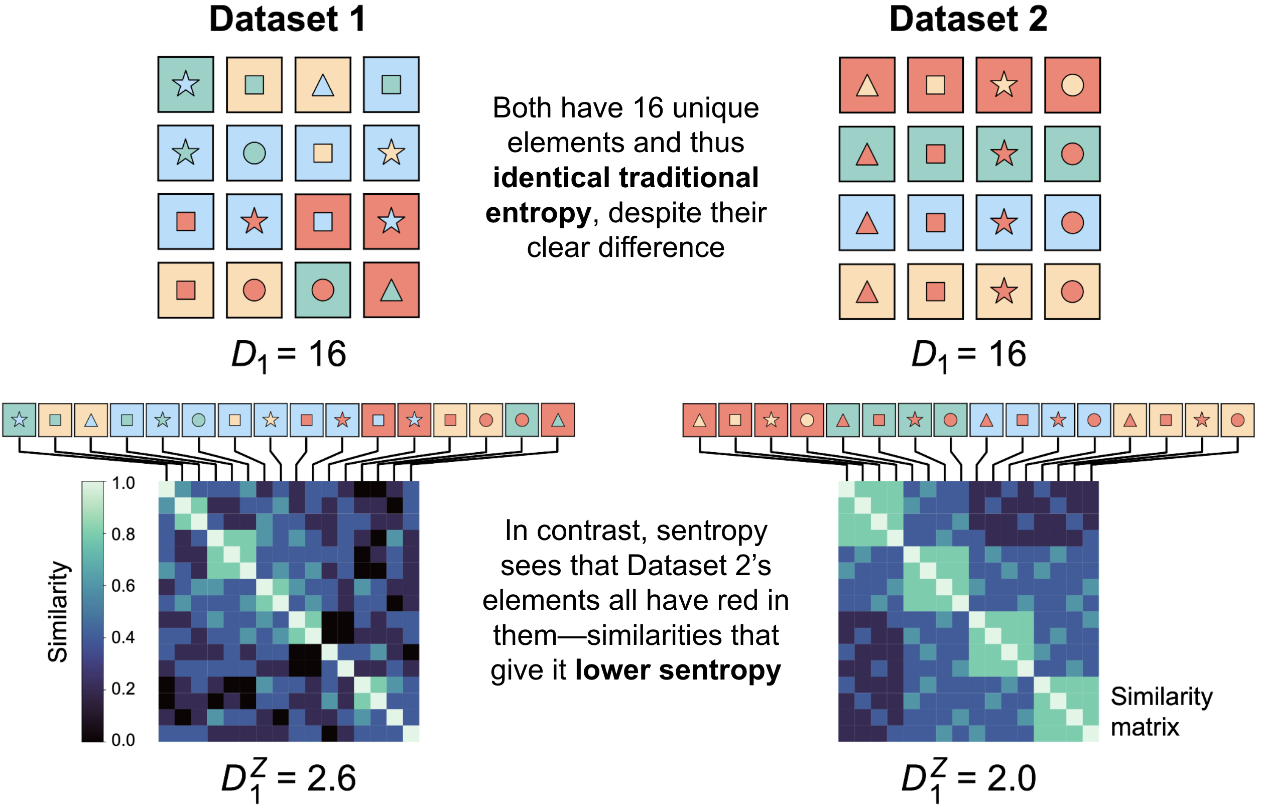
sentropy calculates similarity-sensitive entropies—sentropy—plus Shannon entropy and the other traditional Rényi entropies (of which Shannon entropy is the best known).
Sentropy reveals differences that traditional entropy cannot. Consider two datasets:
Key terms
- Shannon entropy is a weighted sum of the relative probabilities (a.k.a. relative frequencies) of the unique elements in a system (e.g. a dataset), with a special weighting (namely, the log of each probability)
- Rényi entropies generalize Shannon entropy by allowing for different weightings, set by varying the viewpoint parameter q (the log corresponds to q=1)
- sentropy generalizes Rényi entropies by incorporating elements' similarities and differences via a similarity matrix, usually constructed using a similarity function
- Exponentiating traditional entropy yields effective-number a.k.a. D-number forms, which express entropies in the same, natural unit: the effective number of elements present in the dataset
- Higher entropy means more diverse (the "D" in D number)
sentropycalculates multiple sentropic measures, including ɑ, β, ɣ, and 𝜌, at both the subset (class) level and for the overall dataset
For the most complete background currently available, see Leinster 2020 and references therein.
How to cite this work
@misc{nguyen2023textitgreylockpythonpackagemeasuring,
      title={sentropy: A Python Package for Revealing Hidden Differences in Complex Datasets},
      author={Phuc Nguyen and Rohit Arora and Elliot D. Hill and Jasper Braun and Alexandra Morgan and Liza M. Quintana and Gabrielle Mazzoni and Ghee Rye Lee and Rima Arnaout and Ramy Arnaout},
      year={2023},
      eprint={2401.00102},
      archivePrefix={arXiv},
      primaryClass={q-bio.QM},
      url={https://arxiv.org/abs/2401.00102},
}
Installation
sentropy is available via the Python Package Index (PyPI) and on GitHub at https://github.com/ArnaoutLab/sentropy
To install:
pip install sentropy
or for speedups using ray (which as of 31 Dec. 2025 is incompatible with the latest version of Python):
pip install sentropy[ray]
For unit tests (including a coverage report), run:
pip install 'sentropy[tests]'
pytest --pyargs sentropy --cov sentropy
The test suite runs successfully on Macintosh, Windows, and Unix systems. Any errors are most likely due to not having installed ray.
Basic usage
The workhorse function is sentropy.sentropy:
from sentropy import sentropy
Main arguments:
P, a list-like object (e.g. a list, a numpy array) of relative frequencies (or a dictionary of these, one per subset or class; see below)similarity, which can be passed as a matrix or a function; the default is the identity matrix $I$q, the viewpoint parameter; default isq=1.measure, which can bealpha,beta,gamma, or others in the Leinster-Cobbold-Reeve (LCR) framework; the default isalphalevel, which can beoverall(a.k.a.dataset) orsubset(a.k.a.class); the default isoverall
(We recommend running the below in ipython, for maximal readability of the output.)
Shannon entropy
When the similarity matrix is the identity matrix—sentropy's default for similarity—there is no similarity between elements i≠j and sentropy reduces to traditional (Rényi) entropy. At the default q=1, this is Shannon entropy. Therefore passing sentropy only a P yields Shannon entropy, in effective-number form:
from sentropy import sentropy
import numpy as np

P = np.array([0.7, 0.3])          # two unique elements comprising 70% and 30% of this single-class dataset, respectively
D1 = sentropy(P)                  # sentropy *without* similarity at default q (q=1) = Shannon entropy,
                                  #   returned in default effective-number (D-number) form (preferred)
                                  # Equivalent to also including the arguments similarity=np.eye(2), measure="alpha", level="both"
H1 = sentropy(P, eff_no=False)    # traditional, non-effective-number form (eff_no=False)

print(f"D1 = {D1:.2f} elements, which corresponds to H1 = {H1:.2f} nats (= {np.log2(D1):.2f} bits)")
Expected output:
D1 = 1.84 elements, which corresponds to H1 = 0.61 nats (= 0.88 bits)
Intuition behind effective numbers. Suppose instead of the frequencies being (0.7, 0.3) they were (0.999999, 0.000001). The population would consist almost completely of element 1. In an intuitive sense, element 2 "shouldn't count" as much. In this case, the effective-number form would be sentropy(np.array([0.999999, 0.000001])) = 1.00001. (The traditional form would be ~0, at 1e-5 nats or 2e-5 bits.) In contrast, (0.7, 0.3) is far less skewed, and so the effective number is far closer to 2, at 1.84. The effective number would be equal to 2 if the frequencies were equal: (0.5, 0.5).
Shannon-type sentropy
Passing a non-identity similarity matrix (similarity≠I) results in sentropy–here, Shannon-type (i.e. q=1):
from sentropy import sentropy
import numpy as np

P = np.array([0.7, 0.3])                      # same dataset as above (two elements, one class)
S = np.array([                                # similarity matrix
  [1. , 0.2],                                 # 20% similar to each other
  [0.2, 1. ],
  ])
D1Z = sentropy(P, similarity=S)               # D-number form (preferred). Note defaults: level="overall", measure="alpha", q=1.
H1Z = sentropy(P, similarity=S, eff_no=False) # traditional form

print(f"D1Z = {D1Z:.2f} elements, which corresponds to H1Z = {H1Z:.2f} nats")
Expected output:
D1Z = 1.55 elements, which corresponds to H1Z = 0.44 nats
Non-zero similarity between elements 1 and 2 reduces the overall entropy of the system relative to the first example above, in which there was zero similarity between the two elements. This can be thought of as a reduction in diversity (whence the "D" in D-number). The "Z" is a convention that means "non-trivial similarity." In this example, the similarity matrix is a numpy array. It can also be a pandas data frame or various kinds of spicy sparse matrices, e.g. COO or CSR matrices.
Multiple measures and multiple q
To get results for multiple q (e.g. 0, 1, and ∞), multiple measures (e.g. alpha and beta), and/or both levels (overall and subset), pass a list-like object to the relevant argument; sentropy() returns an object with relevant values:
from sentropy import sentropy
import numpy as np

P = np.array([0.7, 0.3])                      # same dataset as above (two elements, one class)
S = np.array([                                # same similarity matrix as above
  [1. , 0.2],
  [0.2, 1. ],
  ])
qs = [0., 1., 2., np.inf]                     # multiple viewpoint parameters
measures = ["alpha", "beta", "gamma"]         # multiple measures
DZ = sentropy(P, similarity=S,                # sentropy...
              q=qs,                           #   ...at multple qs...
              measure=measures)               #   ...for multiple measures
                                              # note when the result of the sentropy() call contains
                                              # multiple values, it returns a function
for measure in measures:
  for q in qs:
    DqZ = DZ(q=q, measure=measure, which='overall') # D-number form (preferred)
    print(f"D{q:.0f}Z {measure}:\t{DqZ:.2f} elements")
  print()
Expected output:
D0Z alpha:	1.60 elements
D1Z alpha:	1.55 elements
D2Z alpha:	1.51 elements
DinfZ alpha:	1.32 elements

D0Z beta:	1.00 elements
D1Z beta:	1.00 elements
D2Z beta:	1.00 elements
DinfZ beta:	1.00 elements

D0Z gamma:	1.60 elements
D1Z gamma:	1.55 elements
D2Z gamma:	1.51 elements
DinfZ gamma:	1.32 elements
Values never rise, and almost always fall, with increasing q. q=0, 1, 2, and ∞ can be thought of as "counting-", "Shannon-", "Simpson-", and "Berger-Parker-type" sentropy, respectively. ɑ=ɣ in this example because there is only one class (see Leinster 2020).
Passing a similarity function
When the similarity matrix would be too large to fit in memory, a function can be passed to similarity, allowing similarilty to be calculated on the fly:
from sentropy import sentropy
import numpy as np

# define a dataset consisting of two amino-acid sequences
elements = np.array(['CARDYW', 'CTRDYW', 'CAKDYW'])     # amino-acid sequences (reminiscent of human IGH CDR3s)
P = np.array([20, 1, 1])                                # the first is present 20 times; the second two are each present once

# define a similarity function where similarity decreases with edit distance between the sequences
from polyleven import levenshtein as edit_distance
def similarity_function(i, j):                          # i, j members of elements
    return 0.3**edit_distance(i, j)

# calculate datset sentropy (at the defaults meausure="alpha" and q=1.)
D1Z = sentropy(P, similarity=similarity_function,
               sfargs=elements)                         # sfargs contains arguments needed by the similarity_function
H1Z = np.log(D1Z)                                       # traditional form (which you could also have returned directly from the sentropy() call with eff_no = False)
print(f"D1Z = {D1Z:.2f} elements, which corresponds to H1Z = {H1Z:.2f} nats")
Expected output:
D1Z = 1.18 elements, which corresponds to H1Z = 0.16 nats
The strings in this example are amino acid sequences, such as might exist in a next-generation sequencing dataset. CARDYW outnumbers the other two 10:1; CTRDYW and CAKDYW might be sequencing errors or mutations. The three sequences are very similar. The combination of these two factors—a big difference in relative frequencies and small differences in sequence—results in this three-element dataset having an effective number of only 1.18 elements.
By default, when a callable is passed to the similarity argument of sentropy, the computation is parallelized with the ray package. In order to turn off the parallelization, pass parallelize=False. If the similarity function is known to be symmetric and that the diagonal entries of the similarity matrix are all 1, a twofold speedup can be obtained by passing symmetric=True.
Furthermore, by default, Ray uses all available CPU cores. To limit it to N cores, initialize Ray yourself before calling sentropy:
import ray
ray.init(num_cpus=N)
Ray keeps its worker processes persistent after the computation finishes, so the memory they occupy is not freed by default. If you prefer to free up that memory, shut Ray down afterwards:
ray.shutdown()
Note that shutting Ray down means the next parallelized computation with sentropy will re-initialize it with all cores again, so you would need to repeat ray.init(num_cpus=N) as well.
Representativeness
Suppose you have a dataset of fruits that has two classes, apples and oranges, and you want to know how representative each class is of the whole dataset. sentropy lets you do this by measuring the representativeness of each class (𝜌, "rho"), which is the reciprocal of β diversity (which measures distinctiveness):
from sentropy import sentropy
import numpy as np

# a dataset with two classes, "apples" and "oranges"
P1 = np.array([12, 3, 0, 0])                  # apples; e.g. 12 Granny Smith and 3 McIntosh (but no oranges)
P2 = np.array([0,  0, 4, 4])                  # oranges; e.g. 4 navel and 4 cara cara (but no apples)
P  = {"apples": P1, "oranges": P2}            # package the classes as P
S = np.array([                                # similarities of all elements, regardless of class
  [1.,  0.7, 0.0, 0.0],                       #    note here the non-zero similarity between apples and oranges
  [0.7, 1.,  0.1, 0.3],
  [0.0, 0.1, 1.,  0.9],
  [0.0, 0.3, 0.9, 1. ],
  ])
D1Z = sentropy(P, similarity=S,
               level="subset",                # level="class" is identical; an alias/synonym
               measure="normalized_rho")
R1 = D1Z(which="apples")                      # note, no need to pass a measure or a viewpoint
R2 = D1Z(which="oranges")                     #    because D1Z only computed 1 measure and 1 viewpoint anyway,
                                              #    since no q (defaulting to q=1) and only one measure were passed
print(f"Normalized rho of Class 1 (apples):  {R1:.2f}")
print(f"Normalized rho of Class 2 (oranges): {R2:.2f}")
Expected output:
Normalized rho of Class 1 (apples):  0.67
Normalized rho of Class 2 (oranges): 0.38
The dataset has more apples, and so the "apples" class (Class 1) is more representative of the dataset.
Results as a pandas dataframe
Same dataset as above, except now results are returned as a dataframe by passing return_dataframe=True:
from sentropy import sentropy
import numpy as np

# a dataset with two classes, "apples" and "oranges"
P1 = np.array([12, 3, 0, 0])              # apples; e.g. 12 Granny Smith and 3 McIntosh (zeros = oranges)
P2 = np.array([0,  0, 4, 4])              # oranges; e.g. 4 navel and 4 cara cara (zeros = apples)
P  = {"apples": P1, "oranges": P2}        # package the classes as P
S = np.array([                            # similarities of all elements, regardless of class
  [1.,  0.7, 0.0, 0.0],                   #    note here the non-zero similarity between apples and oranges
  [0.7, 1.,  0.1, 0.3],
  [0.0, 0.1, 1.,  0.9],
  [0.0, 0.3, 0.9, 1. ],
  ])
D1Z = sentropy(P, similarity=S,
               level="subset",            # level="class" is identical; an alias/synonym
               measure="normalized_rho",
               return_dataframe=True)
display(D1Z)                              # (ipython) sentropies on the diagonals; relative sentropies on the off-diagonals
Expected output:
     level  viewpoint  normalized_rho
0   apples          1        0.669532
1  oranges          1        0.375035
Relative sentropy and cross-sentropy
Shannon-type relative entropy without similarity is called the Kullback-Leibler divergence and is used throughout machine learning (and elsewhere). sentropy lets us calculate the similarity-sensitive version by passing two P arguments:
from sentropy import sentropy
import numpy as np

# a dataset with two classes, "apples" and "oranges"
P1 = np.array([12, 3, 0, 0])              # apples; e.g. 12 Granny Smith and 3 McIntosh (zeros = oranges)
P2 = np.array([0,  0, 4, 4])              # oranges; e.g. 4 navel and 4 cara cara (zeros = apples)
S = np.array([                            # similarities of all elements, regardless of class
  [1.,  0.7, 0.1, 0.1],                   #    note here the non-zero similarity between apples and oranges
  [0.7, 1.,  0.1, 0.3],
  [0.1, 0.1, 1.,  0.9],
  [0.1, 0.3, 0.9, 1. ],
  ])
KLZ_12  = sentropy(P1, P2, similarity=S)  # KL of apples to oranges
KLZ_21  = sentropy(P2, P1, similarity=S)  # KL of oranges to apples (recall, KL is not symmetric)

print("Effective-number form of similarity-sensitive KL divergence (KLZ) of:")
print(f"  apples to oranges: {KLZ_12:.2f}")
print(f"  oranges to apples: {KLZ_21:.2f}")
Expected output:
Effective-number form of similarity-sensitive KL divergence (KLZ) of:
  apples to oranges: 7.84
  oranges to apples: 8.03
If we want to get both directions in a table, we can instead pass a pandas dataframe:
from sentropy import sentropy
import numpy as np
import pandas as pd

# a dataset with two classes, "apples" and "oranges"
P1 = np.array([12, 3, 0, 0])             # apples; e.g. 12 Granny Smith and 3 McIntosh (zeros = oranges)
P2 = np.array([0,  0, 4, 4])             # oranges; e.g. 4 navel and 4 cara cara (zeros = apples)
S = np.array([                           # similarities of all elements, regardless of class
  [1.,  0.7, 0.1, 0.1],                  #    note here the non-zero similarity between apples and oranges
  [0.7, 1.,  0.1, 0.3],
  [0.1, 0.1, 1.,  0.9],
  [0.1, 0.3, 0.9, 1. ],
  ])
P  = {"apples": P1, "oranges": P2}       # package the classes as P
P = pd.DataFrame(P)
KLZ_df = sentropy(P, P, similarity=S,    # return a dataframe with the KLs on the off-diagonals
              level="class",
              return_dataframe=True)

KLZ_arr = sentropy(P, P, similarity=S,   # default returns a numpy array with the KLs on the off-diagonals
                  level="class")

print("As a dataframe:")
display(KLZ_df)
print()
print("As a numpy array:")
print(KLZ_arr)
Expected output:
As a dataframe:
           apples   oranges
apples   1.000000  7.842581
oranges  8.028965  1.000000

As a numpy array:
[[1.         7.84258081]
 [8.02896542 1.        ]]
The syntax to compute the similarity-sensitive analog of the cross entropy is analogous, except that we need to pass measure="sce".
Ordinariness
Suppose you have two datasets of animals. The first dataset consists of fish and ladybugs: a vertebrate and an invertebrate. The second dataset consists of bees, butterflies, and lobsters: all invertebrates. The two datasets are disjoint: there are no fish or ladybugs in the second dataset, and vice versa. However, there are genetic similarities between all these species even though they are in separate datasets. Therefore we can define the similarity between them based on genetic relatedness. Now: suppose you want some measure of how similar each element of the first dataset is to the second dataset, i.e. how much each element would "belong" in the second dataset. This is measured by ordinariness: ladybugs would be more "ordinary" in the second dataset, since ladybugs are invertebrates. Strictly speaking this can be calculated without sentropy:
import numpy as np
P = np.array([5000, 2000, 3000])             # frequencies of a dataset of bees, butterflies, and lobsters, respectively
S_fish    = np.array([0.22, 0.27, 0.28])     # fish's genetic similarities to bee, butterfly, and lobster
S_ladybug = np.array([0.60, 0.55, 0.45])     # ladybug's genetic similarities to each of these
S = np.stack([S_fish, S_ladybug])            # note, a non-square similarity matrix: (ladybug, fish) x (bee, butterfly, lobset)
O_fish, O_ladybug = S @ (P/P.sum())          # ordinariness of fish and ladybugs in the bees/butterflies/lobsters dataset

print("In this bee-butterfly-lobster dataset, with genetics-based similarity, how ordinary would we consider:")
print(f"  a fish?    {O_fish:.2f}")
print(f"  a ladybug? {O_ladybug:.2f}")
Expected output:
In this bee-butterfly-lobster dataset, with genetics-based similarity, how ordinary would we consider:
  a fish?    0.25
  a ladybug? 0.55
but sentropy provides speedup with Ray parallelization:
from sentropy import interset_ordinariness
# Three objects in X whose ordinariness we want to calculate.
X = np.array([
    [1.0, 0.0],
    [0.0, 1.0],
    [0.7, 0.7],
])

# Four objects in the reference set Y.
Y = np.array([
    [1.0, 0.0],
    [0.9, 0.1],
    [0.0, 1.0],
    [0.1, 0.9],
])

# Raw counts for the four elements of Y.
Y_counts = np.array([100, 50, 25, 25])

ordinariness = interset_ordinariness(
    X=X,
    Y=Y,
    Y_abundance=Y_counts,
    similarity=lambda x,y : np.dot(x,y),
)
print(ordinariness)
The expected output is
[0.7375, 0.2625, 0.7]
.
Using torch and the GPU
To utilize torch instead of numpy, pass backend="torch". To have the computation run on the GPU, pass backend="torch" and either device="mps" or device="cuda".
from sentropy import sentropy
import numpy as np

# a dataset with two classes, "apples" and "oranges"
P1 = np.array([12, 3, 0, 0])                  # apples; e.g. 12 Granny Smith and 3 McIntosh (but no oranges)
P2 = np.array([0,  0, 4, 4])                  # oranges; e.g. 4 navel and 4 cara cara (but no apples)
P  = {"apples": P1, "oranges": P2}            # package the classes as P
S = np.array([                                # similarities of all elements, regardless of class
  [1.,  0.7, 0.0, 0.0],                       #    note here the non-zero similarity between apples and oranges
  [0.7, 1.,  0.1, 0.3],
  [0.0, 0.1, 1.,  0.9],
  [0.0, 0.3, 0.9, 1. ],
  ])
D1Z = sentropy(P, similarity=S,
               level="subset",                # level="class" is identical; an alias/synonym
               measure="normalized_rho", backend="torch")
R1 = D1Z(which="apples")                      # note, no need to pass a measure or a viewpoint
R2 = D1Z(which="oranges")                     # because D1Z only computed 1 measure and 1 viewpoint anyway
print("R1 using torch:", R1)
print("R2 using torch:", R2)

D1Z = sentropy(P, similarity=S,
               level="subset",                # level="class" is identical; an alias/synonym
               measure="normalized_rho", backend="torch", device="mps")

R1 = D1Z(which="apples")                      # note, no need to pass a measure or a viewpoint
R2 = D1Z(which="oranges")                     # because D1Z only computed 1 measure and 1 viewpoint anyway
print("R1 using torch and GPU:", R1)
print("R2 using torch and GPU:", R2)
Expected output:
R1 using torch: tensor(0.6695, dtype=torch.float64)
R2 using torch: tensor(0.3750, dtype=torch.float64)
R1 using torch and GPU: tensor(0.6695, device='mps:0')
R2 using torch and GPU: tensor(0.3750, device='mps:0')
Vendi score
This package also computes Vendi scores, which is an alternative definition of similarity-sensitive diversity in addition to the Leinster-Cobbold-Reeve diversity framework. To compute Vendi scores, we simply pass measure='vendi' to the sentropy function.
More applications
In this preprint of ours, we appled sentropy to various fields, including immunomics, metagenomics, medical imaging, and digital pathology. The code for each of these applications is in the following Jupyter notebooks. Please follow along with the paper:
Alternatives
To date, we know of no other python package that implements all the measures defined by Reeve at al.
- packeages in other languages that enable some of the capabilities of
sentropy: R and Julia cdiversitypackage calculates Hill-number diversity but without similarity for immune repertoiresvendi-score: alternative formeasure='vendi'to thesentropyfunction
Release history
- Version 1.5.0: optimized interset ordinariness to include deduplication, redefined Vendi score of overall set not to be the power mean of subsets' Vendi score
- Version 1.4.0: implemented interset ordinariness, auto-tuning Ray hyperparameters, slight improvement to sparse matrix API.
- Version 1.3.0: sped up the SKL computation.
- Version 1.2.0: implemented the Vendi score.
- Version 1.1.0: implemented the similarity-sensitive crossentropy.


Download files
Download the file for your platform. If you're not sure which to choose, learn more about installing packages.
Source Distribution
Built Distribution
Filter files by name, interpreter, ABI, and platform.
If you're not sure about the file name format, learn more about wheel file names.
Copy a direct link to the current filters
File details
Details for the file sentropy-1.5.0.tar.gz.
File metadata
- Download URL: sentropy-1.5.0.tar.gz
- Upload date:
- Size: 2.2 MB
- Tags: Source
- Uploaded using Trusted Publishing? No
- Uploaded via:
twine/7.0.0 CPython/3.12.8
File hashes
| Algorithm | Hash digest | |
|---|---|---|
| SHA256 |
5db65bc206248eca222dd9a68779f03a67928fb3be01c0a06362c4ce227c72d7
|
|
| MD5 |
c93d2c28e811918fb6a86580148fdbe7
|
|
| BLAKE2b-256 |
6bdbffb2d2345d31083fc22c6a49484a9de1f54bf631ca2ebbb9d6b7d9092874
|
File details
Details for the file sentropy-1.5.0-py3-none-any.whl.
File metadata
- Download URL: sentropy-1.5.0-py3-none-any.whl
- Upload date:
- Size: 63.8 kB
- Tags: Python 3
- Uploaded using Trusted Publishing? No
- Uploaded via:
twine/7.0.0 CPython/3.12.8
File hashes
| Algorithm | Hash digest | |
|---|---|---|
| SHA256 |
778b9fb6f38b8d790e0970ccef20bdb9a5f8e3155b081e1f6e4b71fbe240b2f0
|
|
| MD5 |
04f6be94f75c35e5dccaef5d3b30f82e
|
|
| BLAKE2b-256 |
2d6b1e0aa38ba5584a25b7cdb150beda79d6c35a611455daa2e787a2a23c40bd
|














