
SlabNIRT
SlabNIRT is a Python package for processing and analysis of data from normalized impulse response testing (NIRT) of concrete slabs, tunnel linings and other plate-like structures. It covers the whole workflow: importing records, preprocessing signals, calculating attributes, combining repeated measurements at each test point, mapping anomalies and exporting results.
NIRT is used to assess the contact between a structure and the surrounding soil, such as voids or loose soil beneath a slab or behind a tunnel lining, and may also reveal defects within the structure itself. It is a recent modification of the impulse-response method standardized in ASTM C1740. In both methods, a hammer impact mainly excites low-frequency flexural vibrations of the structure, and a sensor records the velocity or acceleration of the response. Where the structure is in good contact with the soil, more vibration energy radiates into the soil and the response decays quickly. Where contact is weakened or lost, less energy is transferred to the soil, so the response typically decays more slowly and its frequency content changes.
The standard method divides the velocity spectrum by the impact-force spectrum, measured with an instrumented hammer, to obtain the mobility of the structure. In contrast, NIRT needs no force measurement, so an ordinary hammer and common single-channel equipment for pile integrity testing can be used. Its attributes describe the decay, frequency content and regularity of the response and do not depend on the strength of the impact: signal energy is calculated from the signal divided by its largest absolute amplitude, spectral attributes describe the shape of the spectrum, and entropy attributes use a tolerance relative to the signal's standard deviation. Anomalies are identified statistically: each attribute value is compared with the survey median, and its deviation is expressed relative to the median absolute deviation (MAD). The method and its applications are described by Churkin et al. (2024a, 2024b), Lozovsky and Churkin (2023, 2025) and Lozovsky et al. (2026) in References.
You can supply your own records as plain text files, including text exports from ZBL instruments and software, or as SEG-Y files recorded with IDS (Logicheskie Sistemy) equipment. A coordinate catalog links the records to their test points for spatial analysis.
Processing and analysis
- Preprocess signals: remove the pre-impact offset, trim records, remove slow drift and low-frequency instrument oscillations, convert acceleration to velocity by integration, normalize signals and calculate their spectra. Optional Butterworth low-pass, high-pass and band-pass filters.
- Calculate attributes: normalized signal energy, peak frequency and spectral centroid, spectral peak width, flatness and normalized area, a band-ratio void index, and sample, multiscale and spectral entropy. See the full list in Attributes.
- Plot signals: show signals, spectra and multiscale entropy curves.
- Combine repeated measurements: calculate a median or mean attribute value at each test point, with standard-error estimates based on the median absolute deviation (MAD) or standard deviation.
- Map attributes and anomalies: display attribute values at test points or as interpolated maps, with optional uncertainty indicators, contours and outlines of the surveyed structure. Colors can show each value's deviation from the survey median in units of 1.4826 × MAD, a robust scale that highlights unusually high or low values.
- Export results: save attributes per record and per test point, signals and spectra as delimited text or Excel files; save figures and a run log.
The workflow consists of functions that you can call in sequence or use separately, selecting preprocessing options, attributes and plot settings for your data. Lozovsky and Churkin (2025) and Lozovsky et al. (2026) describe the processing, statistical analysis and mapping approach, with field and model examples; see References.
Installation
Requires Python 3.12 or newer.
python -m pip install slabnirt
To draw boundaries or other map overlays from shapefiles, install the optional GIS dependency instead:
python -m pip install "slabnirt[shapefiles]"
Quick start
The example and its dataset are in this repository, not in the installed package. Download or clone the repository and run from its root directory:
python examples/slab_model_workflow.py
It runs the full workflow and writes attribute tables, signal and map
figures, the signals and spectra of two sample points, and a run log to
slab_model_output/.
The example uses simulated vertical-velocity records for a 2.8 × 1.9 × 0.17 m concrete slab resting on sand, with an air void under its center. The dataset contains 1788 records at 462 test points. The model and processing settings are described in the example script.
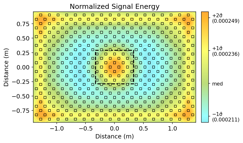
The colors show how far normalized signal energy lies above or below the survey median. One color-scale unit is 1.4826 × MAD, a measure of spread calculated from the test-point values. The dashed rectangle marks the modeled void.
The model is by Ilya Lozovsky, Ruslan Zhostkov and Aleksei Churkin; a paper describing it is in preparation. The bundled records are licensed under CC BY 4.0.
Using your own records
Adapt
the example workflow
by supplying
record files and a coordinate catalog. The package accepts velocity or
acceleration records. To analyze velocity from acceleration measurements,
set integrate_times=1 in preprocess_traces; velocity records need no
integration.
- Text records (
.txt), including ZBL exports: one file per record, with whitespace-separated columns and no header. The first column is time; the remaining columns contain signals. Samples must be uniformly spaced.load_tracesreads the first signal column by default. Time is in seconds; settime_scaling=0.001for exports with time in milliseconds. - Alternatively, SEG-Y records (
.sgy): the format written by IDS (Logicheskie Sistemy) equipment. - Coordinate catalog (CSV or Excel
.xlsx), for either record format: columnsfilename,xandy. Use the record filenames, with or without extensions, and give measurements at the same test point (a site in the function documentation) the same coordinates. Map labels use meters by default.
For velocity records in records/ with time in seconds and a coordinate
catalog named catalog.csv, this example calculates three attributes,
takes their medians at each point, exports the results and draws maps:
from slabnirt import (
    MapPlotConfig,
    average_attributes,
    calculate_signal_parameters,
    export_tracedata,
    load_traces,
    plot_maps,
    preprocess_traces,
    read_coordinates_from_catalog,
)

attrs = ["norm_signal_energy", "normalized_spectrum_area", "spectral_centroid"]
names, x, y = read_coordinates_from_catalog("catalog.csv")
traces = load_traces(
    "txt", "records",
    filenames_with_coordinates=names, x_position=x, y_position=y,
)
processed = preprocess_traces(traces)
calculate_signal_parameters(processed, attrs=attrs, use_power_spectrum=True)
average_attributes(processed, average_algorithm=["median"])
export_tracedata(
    processed, mode=["attributes", "attributes_avg"], output_dir="results",
)
plot_maps(processed, MapPlotConfig(
    attrs_to_plot=attrs, color_norm="mad-scaled", output_dir="results",
    show=False,
))
Function docstrings describe the settings and returned data, for example
help(preprocess_traces) and help(calculate_signal_parameters).
Attributes
| Attribute | Definition |
|---|---|
norm_signal_energy |
Area under the squared, peak-normalized signal as a function of time (s) |
normalized_spectrum_area |
Area under the peak-normalized spectrum as a function of frequency (Hz) |
spectral_centroid |
Weighted mean frequency, using spectral values at or above a chosen fraction of the peak (Hz) |
norm_spectrum_area_over_centroid |
Normalized spectrum area divided by spectral centroid |
peak_frequency |
Frequency at which the spectrum has its largest value (Hz) |
spectral_peak_width |
Width of the main spectral peak between its half-power points, divided by twice the peak frequency |
spectral_flatness |
Geometric mean of spectral power divided by its arithmetic mean |
void_index |
Largest spectral value in one frequency band divided by the median or mean value in another |
sampen |
Sample entropy, calculated using the Richman–Moorman algorithm (2000) |
MSE |
Refined composite multiscale entropy (RCMSE), using the Wu et al. (2014) algorithm; returns values at each scale and their mean over finite values |
spectral_entropy |
Shannon entropy of the spectral power distribution, normalized to 0–1: 0 for power in one frequency bin, 1 for equal power in all selected bins |
Normalized spectrum area has units of Hz because it integrates a dimensionless spectrum over frequency. The half-power points used for peak width are the frequencies on either side of the peak where power falls to half its maximum.
The examples explicitly use use_power_spectrum=True for spectral
attributes, following Lozovsky and Churkin (2025). Power is also the
function default; set use_power_spectrum=False to use amplitude spectra.
Spectral flatness and spectral entropy use power in either mode.
freq_range selects the analysis band; void_index has separate band
settings.
Citation and license
To cite SlabNIRT, use CITATION.cff. The package is licensed under BSD-3-Clause.
References
Normalized impulse response testing and its attributes:
- Churkin A.A., Kapustin V.V., Pleshko M.S. Normalized impulse response testing in underground constructions monitoring. Journal of Mining Institute. 2024a. Vol. 270. Pp. 963–976.
- Churkin A.A., Lozovsky I.N., Volodin G.V., Zhostkov R.A. Evaluating the Integrity of Slab–Soil Contact with Impulse Response Testing: Insights from Numerical Simulations. Soil Mechanics and Foundation Engineering. 2024b. Vol. 61. Pp. 62–67. DOI
- Lozovsky I.N., Churkin A.A. Multiscale Entropy Analysis for Slab Impulse Response Testing. Bulletin of the Russian Academy of Sciences: Physics. 2023. Vol. 87. No. 10. Pp. 1518–1522. DOI
- Lozovsky I.N., Churkin A.A. New approaches to processing and analysis of data from normalized impulse response testing of reinforced concrete slabs. Earthquake Engineering. Constructions Safety. 2025. No. 4. Pp. 69–85. (In Russian) DOI
- Lozovsky I.N., Churkin A.A., Zhostkov R.A. Impulse response testing of tunnel linings using entropy analysis: a numerical and experimental study. Defektoskopiya / Russian Journal of Nondestructive Testing. 2026. No. 10. Pp. 15–29. (In Russian; accepted for publication)
Entropy algorithms:
- Richman J.S., Moorman J.R. Physiological time-series analysis using approximate entropy and sample entropy. American Journal of Physiology-Heart and Circulatory Physiology. 2000. Vol. 278. No. 6. Pp. H2039–H2049. DOI
- Wu S.-D., Wu C.-W., Lin S.-G. et al. Analysis of complex time series using refined composite multiscale entropy. Physics Letters A. 2014. Vol. 378. No. 20. Pp. 1369–1374. DOI
1 maintainer

Release files for slabnirt 0.7.0
For a detailed explanation of source distributions (sdists) and built distributions (wheels), please see the package formats documentation.
Source distribution (sdist)
| File | Size | Uploaded | |
|---|---|---|---|
| slabnirt-0.7.0.tar.gz | 3.4 MB | Details |
Built distribution (wheel)
| File | Interpreter | ABI | Platform | Reset |
|---|---|---|---|---|
| slabnirt-0.7.0-py3-none-any.whl | Python 3 | none | any | Details |
Total release size: 3.5 MB
Release files / slabnirt-0.7.0.tar.gz
| Download URL | slabnirt-0.7.0.tar.gz |
|---|---|
| Size | 3.4 MB |
| Tags | Source |
|
SHA-256 checksum How to use checksums |
4795d637a334150bfae5acaf98117e337bc0fa75c7abd48ae579f5e485809c9e
|
|
BLAKE2b-256 checksum How to use checksums |
d6193e450ede3af5bf49a6b4223532c7922d100edbd9e567fd70987cc63e394d
|
| Upload date | |
|
Uploaded using Trusted Publishing? What is trusted publishing? |
Yes |
| Uploaded via |
twine/7.0.0 CPython/3.13.14
|
Provenance
Provenance describes where a file came from. On PyPI, provenance is shared via attestations, which provide a verifiable record of the build or publishing details. View details, limitations and caveats.


PyPI Publish Attestation
PyPI verified that this artifact, at this checksum, originated from the publisher listed below.
Signed by GitHub Actions, verified by PyPI on Sep 25, 2026.
Transparency logRelease files / slabnirt-0.7.0-py3-none-any.whl
| Download URL | slabnirt-0.7.0-py3-none-any.whl |
|---|---|
| Size | 64.5 kB |
| Tags | Python 3 |
|
SHA-256 checksum How to use checksums |
f523ea6a235a2cb560c6b6c32c93ee22529af8b28e6f9ea7bfd16ef113d0ffe6
|
|
BLAKE2b-256 checksum How to use checksums |
c6b19f0cb0f8bac2bbf803bfb4b2b4c2a81832c338e02bc03d733e16a3ea70df
|
| Upload date | |
|
Uploaded using Trusted Publishing? What is trusted publishing? |
Yes |
| Uploaded via |
twine/7.0.0 CPython/3.13.14
|
Provenance
Provenance describes where a file came from. On PyPI, provenance is shared via attestations, which provide a verifiable record of the build or publishing details. View details, limitations and caveats.
PyPI Publish Attestation
PyPI verified that this artifact, at this checksum, originated from the publisher listed below.
Signed by GitHub Actions, verified by PyPI on Sep 25, 2026.
Transparency log












