Data loader for Solar Orbiter/EPD energetic charged particle sensors EPT, HET, and STEP.

Project description


Python data loader for Solar Orbiter’s (SolO) Energetic Particle Detector (EPD). At the moment provides level 2 (l2), level 3 (l3), and low latency (ll) data (more details on data levels here) obtained through CDF files from ESA’s Solar Orbiter Archive (SOAR) for the following sensors:
Electron Proton Telescope (EPT)
High Energy Telescope (HET)
SupraThermal Electrons and Protons (STEP)
Current caveats:
Only the standard rates data products are supported (i.e., no burst or high cadence data).
For EPT and HET, only electrons, protons and alpha particles are processed (i.e., for HET He3, He4, C, N, O, Fe are omitted at the moment).
For STEP, electron data needs to be calculated manually.
The Suprathermal Ion Spectrograph (SIS) is not yet included.
Disclaimer
This software is provided “as is”, with no guarantee. It is no official data source, and not officially endorsed by the corresponding instrument teams. Please always refer to the official EPD data description before using the data!
Installation
solo_epd_loader requires python >= 3.9.
It can be installed either from PyPI using:
pip install solo-epd-loaderor from Anaconda using:
conda install -c conda-forge solo-epd-loaderUsage
The standard usecase is to utilize the epd_load function, which returns Pandas dataframe(s) of the EPD measurements and a dictionary containing information on the energy channels.
from solo_epd_loader import epd_load

df_1, df_2, energies = epd_load(sensor, startdate, enddate=None, level='l2', viewing=None, path=None,
                                autodownload=False, only_averages=False)
Input
sensor: 'ept', 'het', or 'step' (string)
startdate, enddate: Datetime object (e.g., dt.date(2021,12,31) or dt.datetime(2021,4,15)) or integer of the form yyyymmdd with empty positions filled with zeros, e.g. 20210415 (if no enddate is provided, enddate = startdate will be used)
level: 'l2' or 'll' (string); defines level of data product: level 2 ('l2'), level 3 ('l3'), or low-latency ('ll'). By default 'l2'.
viewing: 'sun', 'asun', 'north', 'south', 'omni' (string) or None; not needed for sensor = 'step'. 'omni' is just calculated as the average of the other four viewing directions: ('sun'+'asun'+'north'+'south')/4
path: directory in which Solar Orbiter data is/should be organized; e.g. '/home/userxyz/solo/data/' (string). See Data folder structure for more details.
autodownload: if True, will try to download missing data files from SOAR (bolean)
only_averages: If True, will for STEP only return the averaged fluxes, and not the data of each of the 15 Pixels. This will reduce the memory consumption. By default False.
Return
For sensor = 'ept' or 'het':
Pandas dataframe with proton fluxes and errors (for EPT also alpha particles) in ‘particles / (s cm^2 sr MeV)’
Pandas dataframe with electron fluxes and errors in ‘particles / (s cm^2 sr MeV)’
Dictionary with energy information for all particles:
String with energy channel info
Value of lower energy bin edge in MeV
Value of energy bin width in MeV
For sensor = 'step':
Pandas dataframe with fluxes and errors in ‘particles / (s cm^2 sr MeV)’
Dictionary with energy information for all particles:
String with energy channel info
Value of lower energy bin edge in MeV
Value of energy bin width in MeV
SupraThermal Electron Proton (STEP) sensor electron measurements
Please note that the STEP electron measurements are not directly provided in the publically released data, but need to be calculated from them. This process is not straightforward, and the resulting data is prone to uncertainties (like contamination). Thus it should only be used scientifically with caution! Please refer to the official EPD data description before using the data!
Data folder structure
The path variable provided to the module should be the base directory where the corresponding cdf data files should be placed in subdirectories. First subfolder defines the data product level (l2, l3, or low_latency at the moment), the next one the instrument (so far only epd), and finally the sensor (ept, het or step).
For example, the folder structure could look like this: /home/userxyz/solo/data/l2/epd/het. In this case, you should call the loader with path='/home/userxyz/solo/data'; i.e., the base directory for the data.
You can use the (automatic) download function described in the following section to let the subfolders be created initially automatically. NB: It might be that you need to run the code with sudo or admin privileges in order to be able to create new folders on your system.
Data download within Python
While using epd_load() to obtain the data, one can choose to automatically download missing data files from SOAR directly from within python. They are saved in the folder provided by the path argument (see above). For that, just add autodownload=True to the function call:
from solo_epd_loader import epd_load

df_protons, df_electrons, energies = \
    epd_load(sensor='het', level='l2', startdate=20200820,
             enddate=20200821, viewing='sun',
             path='/home/userxyz/solo/data/', autodownload=True)

# plot protons and alphas
ax = df_protons.plot(logy=True, subplots=True, figsize=(20,60))
plt.show()

# plot electrons
ax = df_electrons.plot(logy=True, subplots=True, figsize=(20,60))
plt.show()
Note: The code will always download the latest version of the file available at SOAR. So in case a file V01.cdf is already locally present, V02.cdf will be downloaded nonetheless.
Example 1 - low latency data
Example code that loads low latency (ll) electron and proton (+alphas) fluxes (and errors) for EPT NORTH telescope from Apr 15 2021 to Apr 16 2021 into two Pandas dataframes (one for protons & alphas, one for electrons). In general available are ‘sun’, ‘asun’, ‘north’, ‘south’, and ‘omni’ viewing directions for ‘ept’ and ‘het’ telescopes of SolO/EPD.
from matplotlib import pyplot as plt
from solo_epd_loader import epd_load

df_protons, df_electrons, energies = \
    epd_load(sensor='ept', level='ll', startdate=20210415,
             enddate=20210416, viewing='north',
             path='/home/userxyz/solo/data/')

# plot protons and alphas
ax = df_protons.plot(logy=True, subplots=True, figsize=(20,60))
plt.show()

# plot electrons
ax = df_electrons.plot(logy=True, subplots=True, figsize=(20,60))
plt.show()
Example 2 - level 2 data
Example code that loads level 2 (l2) electron and proton (+alphas) fluxes (and errors) for HET SUN telescope from Aug 20 2020 to Aug 20 2020 into two Pandas dataframes (one for protons & alphas, one for electrons).
from matplotlib import pyplot as plt
from solo_epd_loader import epd_load
df_protons, df_electrons, energies = \
epd_load(sensor='het', level='l2', startdate=20200820,
enddate=20200821, viewing='sun',
path='/home/userxyz/solo/data/')
# plot protons and alphas
ax = df_protons.plot(logy=True, subplots=True, figsize=(20,60))
plt.show()
# plot electrons
ax = df_electrons.plot(logy=True, subplots=True, figsize=(20,60))
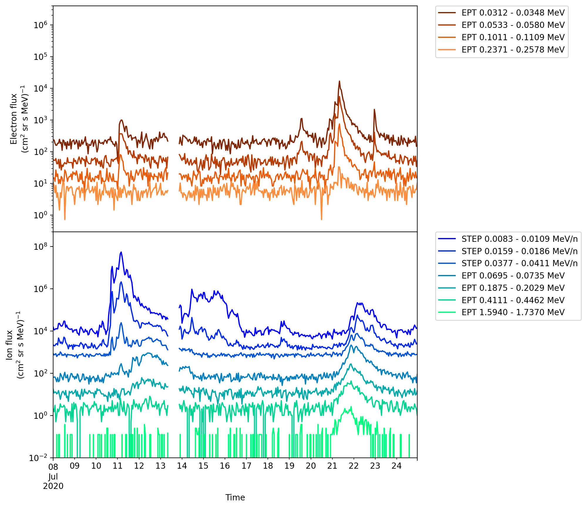
plt.show()Example 3 - partly reproducing Fig. 2 from Gómez-Herrero et al. 2021 [1]
from matplotlib import pyplot as plt
from solo_epd_loader import epd_load
import numpy as np

# set your local path here
lpath = '/home/userxyz/solo/data'

# load ept sun viewing data
df_protons_ept, df_electrons_ept, energies_ept = \
   epd_load(sensor='ept', level='l2', startdate=20200708,
            enddate=20200724, viewing='sun', path=lpath, autodownload=True)

# load step data
df_step, energies_step = \
   epd_load(sensor='step', level='l2', startdate=20200708,
            enddate=20200724, path=lpath, autodownload=True)

# change time resolution to get smoother curve (resample with mean)
resample = '60min'

fig, axs = plt.subplots(2, sharex=True, figsize=(8, 10), dpi=200)
axs[0].set_prop_cycle('color', plt.cm.Oranges_r(np.linspace(0,1,7)))
axs[1].set_prop_cycle('color', plt.cm.winter(np.linspace(0,1,7)))

# plot selection of ept electron channels
for channel in [0, 8, 16, 26]:
   df_electrons_ept['Electron_Flux'][f'Electron_Flux_{channel}'].resample(resample).mean().plot(
      ax = axs[0], logy=True, label='EPT '+energies_ept["Electron_Bins_Text"][channel][0])

# plot selection of step ion channels
for channel in [8, 17, 33]:
   df_step[f'Magnet_Avg_Flux_{channel}'].resample(resample).mean().plot(
      ax = axs[1], logy=True, label='STEP '+energies_step["Bins_Text"][channel][0])

# plot selection of ept ion channels
for channel in [6, 22, 32, 48]:
   df_protons_ept['Ion_Flux'][f'Ion_Flux_{channel}'].resample(resample).mean().plot(
      ax = axs[1], logy=True, label='EPT '+energies_ept["Ion_Bins_Text"][channel][0])

axs[0].set_ylim([0.3, 4e6])
axs[1].set_ylim([0.01, 5e8])

axs[0].set_ylabel("Electron flux\n"+r"(cm$^2$ sr s MeV)$^{-1}$")
axs[1].set_ylabel("Ion flux\n"+r"(cm$^2$ sr s MeV)$^{-1}$")
axs[0].legend(bbox_to_anchor=(1.05, 1), loc=2, borderaxespad=0.)
axs[1].legend(bbox_to_anchor=(1.05, 1), loc=2, borderaxespad=0.)
plt.subplots_adjust(hspace=0)
fig.savefig("gh2021_fig_2.png", bbox_inches = "tight")
plt.close('all')
NB: This is just an approximate reproduction with different energy
channels, different time resolution, and different viewing direction!
Note also that the STEP data can not be used straightforwardly.
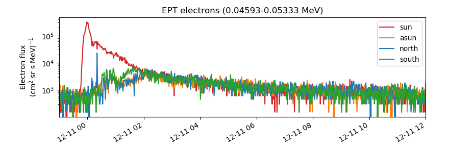
Example 4 - partly reproducing Fig. 2e from Wimmer-Schweingruber et al. 2021 [2]
from matplotlib import pyplot as plt
from solo_epd_loader import epd_load
import datetime
import pandas as pd

# set your local path here
lpath = '/home/userxyz/solo/data'

# load data
df_protons_sun, df_electrons_sun, energies = \
    epd_load(sensor='ept', level='l2', startdate=20201210,
             enddate=20201211, viewing='sun',
             path=lpath, autodownload=True)
df_protons_asun, df_electrons_asun, energies = \
    epd_load(sensor='ept', level='l2', startdate=20201210,
             enddate=20201211, viewing='asun',
             path=lpath, autodownload=True)
df_protons_south, df_electrons_south, energies = \
    epd_load(sensor='ept', level='l2', startdate=20201210,
             enddate=20201211, viewing='south',
             path=lpath, autodownload=True)
df_protons_north, df_electrons_north, energies = \
    epd_load(sensor='ept', level='l2', startdate=20201210,
             enddate=20201211, viewing='north',
             path=lpath, autodownload=True)

# plot mean intensities of two energy channels; 'channel' defines the lower one
channel = 6
ax = pd.concat([df_electrons_sun['Electron_Flux'][f'Electron_Flux_{channel}'],
                df_electrons_sun['Electron_Flux'][f'Electron_Flux_{channel+1}']],
                axis=1).mean(axis=1).plot(logy=True, label='sun', color='#d62728')
ax = pd.concat([df_electrons_asun['Electron_Flux'][f'Electron_Flux_{channel}'],
                df_electrons_asun['Electron_Flux'][f'Electron_Flux_{channel+1}']],
                axis=1).mean(axis=1).plot(logy=True, label='asun', color='#ff7f0e')
ax = pd.concat([df_electrons_north['Electron_Flux'][f'Electron_Flux_{channel}'],
                df_electrons_north['Electron_Flux'][f'Electron_Flux_{channel+1}']],
                axis=1).mean(axis=1).plot(logy=True, label='north', color='#1f77b4')
ax = pd.concat([df_electrons_south['Electron_Flux'][f'Electron_Flux_{channel}'],
                df_electrons_south['Electron_Flux'][f'Electron_Flux_{channel+1}']],
                axis=1).mean(axis=1).plot(logy=True, label='south', color='#2ca02c')

plt.xlim([datetime.datetime(2020, 12, 10, 23, 0),
          datetime.datetime(2020, 12, 11, 12, 0)])

ax.set_ylabel("Electron flux\n"+r"(cm$^2$ sr s MeV)$^{-1}$")
plt.title('EPT electrons ('+str(energies['Electron_Bins_Low_Energy'][channel])
          + '-' + str(energies['Electron_Bins_Low_Energy'][channel+2])+' MeV)')
plt.legend()
plt.show()
NB: This is just an approximate reproduction; e.g., the channel
combination is a over-simplified approximation!
Example 5 - EPT level 3 data
Example code that loads level 3 (l3) electron and ion fluxes (and errors) for the EPT sensor for the GLE event on Oct 28 2024.
Note that for EPT level 3 data, all particle species and viewing directions are saved in a single Pandas dataframe that also includes pitch-angle distributions. In addition, two additional dataframes are provided, which provide the particle flow directions (unit vector) in RTN coordinates as well as spacecraft coordinate information. Also, next to a dictionary providing energy information, another dictionary is returned that contains the CDF file metadata. See data.serpentine-h2020.eu/l3data/solo/ for more details on the data product.
Also note that the corrected electron fluxes can contain negative values. Though the user probably wants to omit them while plotting, they need to be included if the data is integrated over time!
from matplotlib import pyplot as plt
from solo_epd_loader import epd_load

df, df_rtn, df_hci, energies, metadata = epd_load(sensor='ept', level='l3',
                                                  startdate=20211028, enddate=20211028,
                                                  autodownload=True, pos_timestamp='start',
                                                  path='/home/userxyz/solo/data/')

# plot ions of south viewing (D stands for "down")
ax = df.filter(like='Ion_Flux_D').plot(logy=True)
plt.show()

# plot electrons for sun viewing
ax = df.filter(like='Electron_Corrected_Flux_S').plot(logy=True)
plt.show()

# plot pitch angles for all four viewings
for v in ['Pitch_Angle_A', 'Pitch_Angle_S', 'Pitch_Angle_N', 'Pitch_Angle_D']:
   ax = df[v].plot(label=v)
plt.legend()
plt.show()
Contributing
Contributions to this package are very much welcome and encouraged! Contributions can take the form of issues to report bugs and request new features or pull requests to submit new code.
References
License
This project is Copyright (c) Jan Gieseler and licensed under the terms of the BSD 3-clause license. This package is based upon the Openastronomy packaging guide which is licensed under the BSD 3-clause license. See the licenses folder for more information.
Acknowledgements
The development of this software has received funding from the European Union’s Horizon 2020 research and innovation programme under grant agreement No 101004159 (SERPENTINE).
Release history Release notifications | RSS feed


Download files
Download the file for your platform. If you're not sure which to choose, learn more about installing packages.
Source Distribution
Built Distribution
Filter files by name, interpreter, ABI, and platform.
If you're not sure about the file name format, learn more about wheel file names.
Copy a direct link to the current filters
File details
Details for the file solo_epd_loader-0.4.4.tar.gz.
File metadata
- Download URL: solo_epd_loader-0.4.4.tar.gz
- Upload date:
- Size: 1.1 MB
- Tags: Source
- Uploaded using Trusted Publishing? No
- Uploaded via: twine/6.1.0 CPython/3.12.5
File hashes
| Algorithm | Hash digest | |
|---|---|---|
| SHA256 |
6fb94173376d520a8a62fa254f730bde335e242e3b73b7dae185d4821b4ec223
|
|
| MD5 |
7fb42df88c0aead0fa1beafe1516c094
|
|
| BLAKE2b-256 |
678d577a09bd5eb159ba5b09aa6ad41f4e11503f5c8f171f3b92b92661978001
|
File details
Details for the file solo_epd_loader-0.4.4-py3-none-any.whl.
File metadata
- Download URL: solo_epd_loader-0.4.4-py3-none-any.whl
- Upload date:
- Size: 452.1 kB
- Tags: Python 3
- Uploaded using Trusted Publishing? No
- Uploaded via: twine/6.1.0 CPython/3.12.5
File hashes
| Algorithm | Hash digest | |
|---|---|---|
| SHA256 |
4c8e7a628b01c68bb205a799412dc82e40e031b00ee0bba3c9d756c59527c08a
|
|
| MD5 |
0cceac1964986e7cbae64ddddb5e08b5
|
|
| BLAKE2b-256 |
d412a0a57c5ec16f3d790c9712ec87bc090598d038c376dc157d006829296b70
|


