Python implementation of solvers for differential algebraic equations (DAEs) and implicit differential equations (IDEs).

Project description
solve_dae - solving differential algebraic equations (DAEs) and implicit differential equations (IDEs) in Python


Python implementation of solvers for differential algebraic equations (DAEs) and implicit differential equations (IDEs) that should be added to scipy one day.
Currently, two different methods are implemented.
- Implicit Radau IIA methods of order 2s - 1 with arbitrary number of odd stages.
- Implicit backward differentiation formula (BDF) of variable order with quasi-constant step-size and stability/ accuracy enhancement using numerical differentiation formula (NDF).
More information about both methods are given in the specific class documentation.
To pique your curiosity
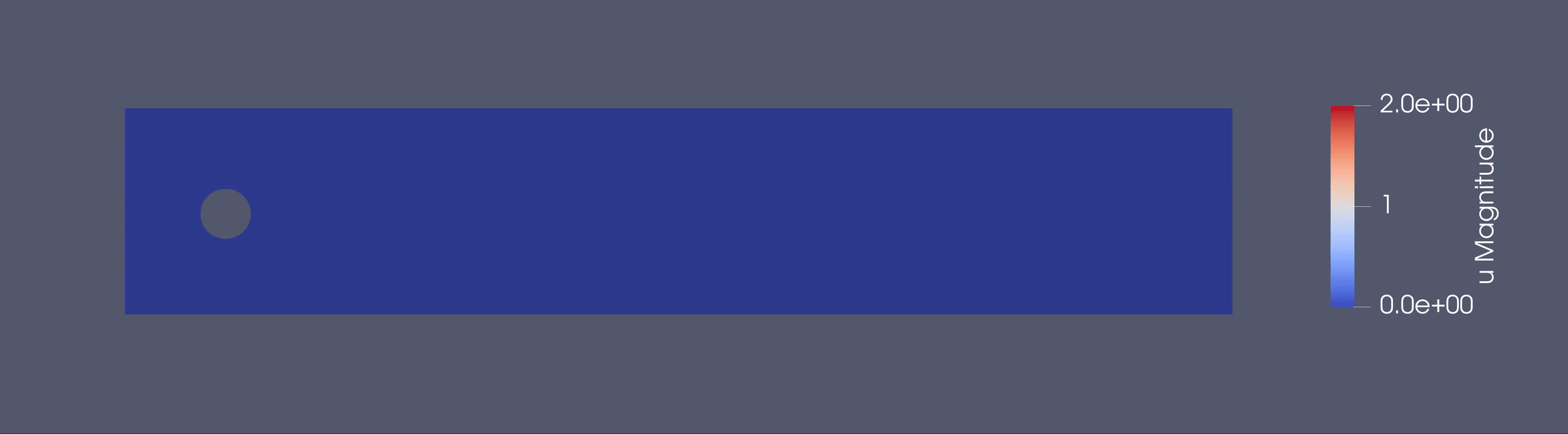
The Kármán vortex street solved by a finite element discretization of the weak form of the incompressible Navier-Stokes equations using FEniCS and the three stage Radau IIA method.
Basic usage
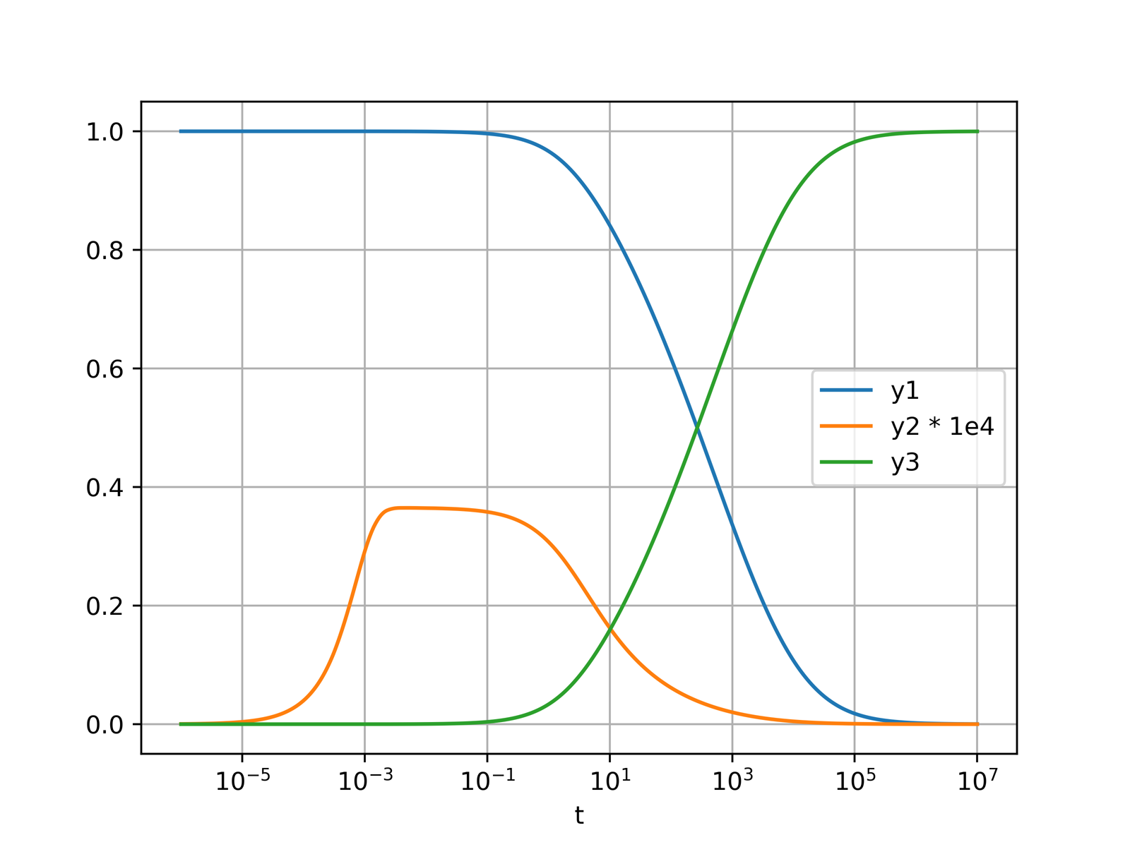
The Robertson problem of semi-stable chemical reaction is a simple system of differential algebraic equations of index 1. It demonstrates the basic usage of the package.
import numpy as np
import matplotlib.pyplot as plt
from solve_dae.integrate import solve_dae


def F(t, y, yp):
    """Define implicit system of differential algebraic equations."""
    y1, y2, y3 = y
    y1p, y2p, y3p = yp

    F = np.zeros(3, dtype=np.common_type(y, yp))
    F[0] = y1p - (-0.04 * y1 + 1e4 * y2 * y3)
    F[1] = y2p - (0.04 * y1 - 1e4 * y2 * y3 - 3e7 * y2**2)
    F[2] = y1 + y2 + y3 - 1 # algebraic equation

    return F


# time span
t0 = 0
t1 = 1e7
t_span = (t0, t1)
t_eval = np.logspace(-6, 7, num=1000)

# initial conditions
y0 = np.array([1, 0, 0], dtype=float)
yp0 = np.array([-0.04, 0.04, 0], dtype=float)

# solver options
method = "Radau"
# method = "BDF" # alternative solver
atol = rtol = 1e-6

# solve DAE system
sol = solve_dae(F, t_span, y0, yp0, atol=atol, rtol=rtol, method=method, t_eval=t_eval)
t = sol.t
y = sol.y

# visualization
fig, ax = plt.subplots()
ax.plot(t, y[0], label="y1")
ax.plot(t, y[1] * 1e4, label="y2 * 1e4")
ax.plot(t, y[2], label="y3")
ax.set_xlabel("t")
ax.set_xscale("log")
ax.legend()
ax.grid()
plt.show()
Advanced usage
More examples are given in the examples directory, which includes
- ordinary differential equations (ODEs)
- differential algebraic equations (DAEs)
- implicit differential equations (IDEs)
Work-precision
In order to investigate the work precision of the implemented solvers, we use different DAE examples with differentiation index 1, 2 and 3 as well as IDE examples.
Index 1 DAE - Brenan
Brenan's index 1 problem is described by the system of differential algebraic equations
$$ \begin{aligned} \dot{y}_1 - t \dot{y}_2 &= y_1 - (1 + t) y_2 \ 0 &= y_2 - \sin(t) . \end{aligned} $$
For the consistent initial conditions $t_0 = 0$, $y_1(t_0) = 1$, $y_2(t_0) = 0$, $\dot{y}_1 = -1$ and $\dot{y}_2 = 1$, the analytical solution is given by $y_1(t) = e^{-t} + t \sin(t)$ and $y_2(t) = \sin(t)$.
This problem is solved for $atol = rtol = 10^{-(1 + m / 4)}$, where $m = 0, \dots, 45$. The resulting error at $t_1 = 10$ is compared with the elapsed time of the used solvers in the figure below. For reference, the work-precision diagram of sundials IDA solver is also added. Note that the elapsed time is scaled by a factor of 100 since the sundials C-code is way faster.
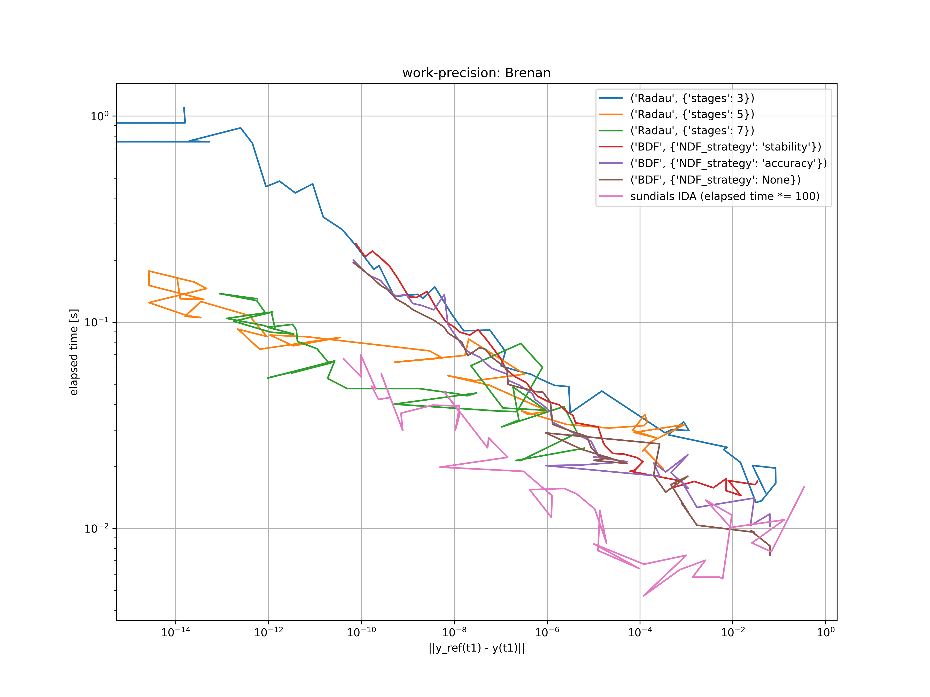
Clearly, the family of Radau IIA methods outplay the BDF/NDF methods for low tolerances. For medium to high tolerances, both methods are appropriate.
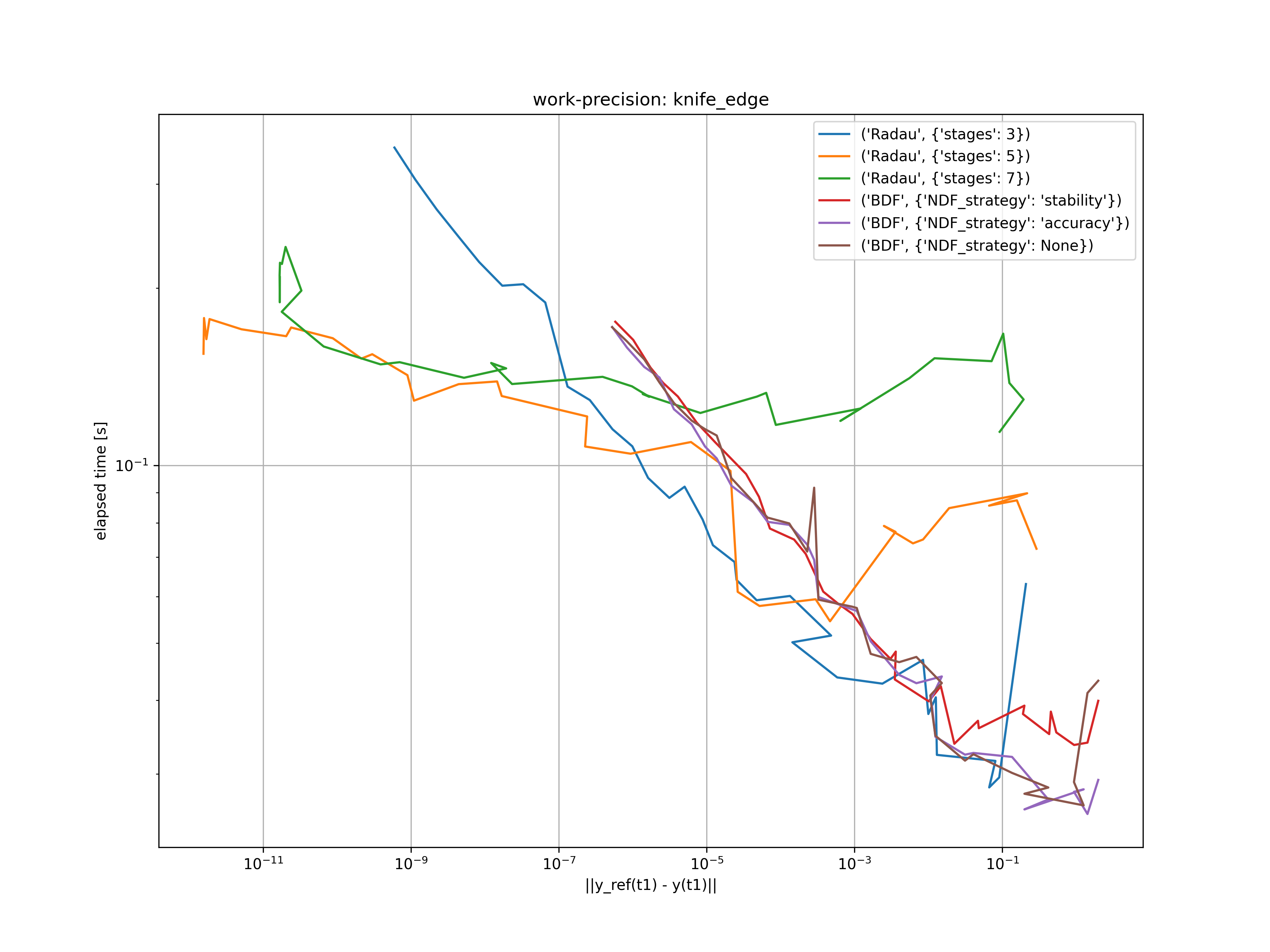
Index 2 DAE - knife edge
The knife edge index 2 problem is a simple mechanical example with nonholonomic constraint. It is described by the system of differential algebraic equations
$$ \begin{aligned} \dot{x} &= u \ \dot{y} &= v \ \dot{\varphi} &= \omega \ m \dot{u} &= m g \sin\alpha + \sin\varphi \lambda \ m \dot{v} &= -\cos\varphi \lambda \ J \dot{\omega} &= 0 \ 0 &= u \sin\varphi - v \cos\varphi . \end{aligned} $$
Since the implemented solvers are designed for index 1 DAEs we have to perform some sort of index reduction. Therefore, we transform the semi-explicit form into a general form as proposed by Gear. The resulting index 1 system is given as
$$ \begin{aligned} \dot{x} &= u \ \dot{y} &= v \ \dot{\varphi} &= \omega \ m \dot{u} &= m g \sin\alpha + \sin\varphi \dot{\Lambda} \ m \dot{v} &= -\cos\varphi \dot{\Lambda} \ J \dot{\omega} &= 0 \ 0 &= u \sin\varphi - v \cos\varphi . \end{aligned} $$
For the initial conditions $t_0 = 0$, $x(t_0) = \dot{x}(t_0) = y(t_0) = \dot{y}(t_0) = \varphi(t_0) = 0$ and $\dot{\varphi}(t_0) = \Omega$, a closed form solution is given by
$$ \begin{aligned} x(t) &= \frac{g \sin\alpha}{2 \Omega^2} \sin^2(\Omega t) \ y(t) &= \frac{g \sin\alpha}{2 \Omega^2} \left(\Omega t - \frac{1}{2}\sin(2 \Omega t)\right) \ \varphi(t) &= \Omega t \ u(t) &= \frac{g \sin\alpha}{\Omega} \sin(\Omega t) \cos(\Omega t) \ v(t) &= \frac{g \sin\alpha}{2 \Omega} \left(1 - \cos(2 \Omega t)\right) = \frac{g \sin\alpha}{\Omega} \sin^2(\Omega t) \ \omega(t) &= \Omega \ \Lambda(t) &= \frac{2g \sin\alpha}{\Omega} (\cos(\Omega t) - 1) , % (2 * m * g * salpha / Omega) * (np.cos(Omega * t) - 1) \end{aligned} $$
with the Lagrange multiplier $\dot{\Lambda}(t) = - 2g \sin\alpha \sin(\Omega t)$.
This problem is solved for $atol = rtol = 10^{-(1 + m / 4)}$, where $m = 0, \dots, 32$. The resulting error at $t_1 = 2 \pi / \Omega$ is compared with the elapsed time of the used solvers in the figure below.
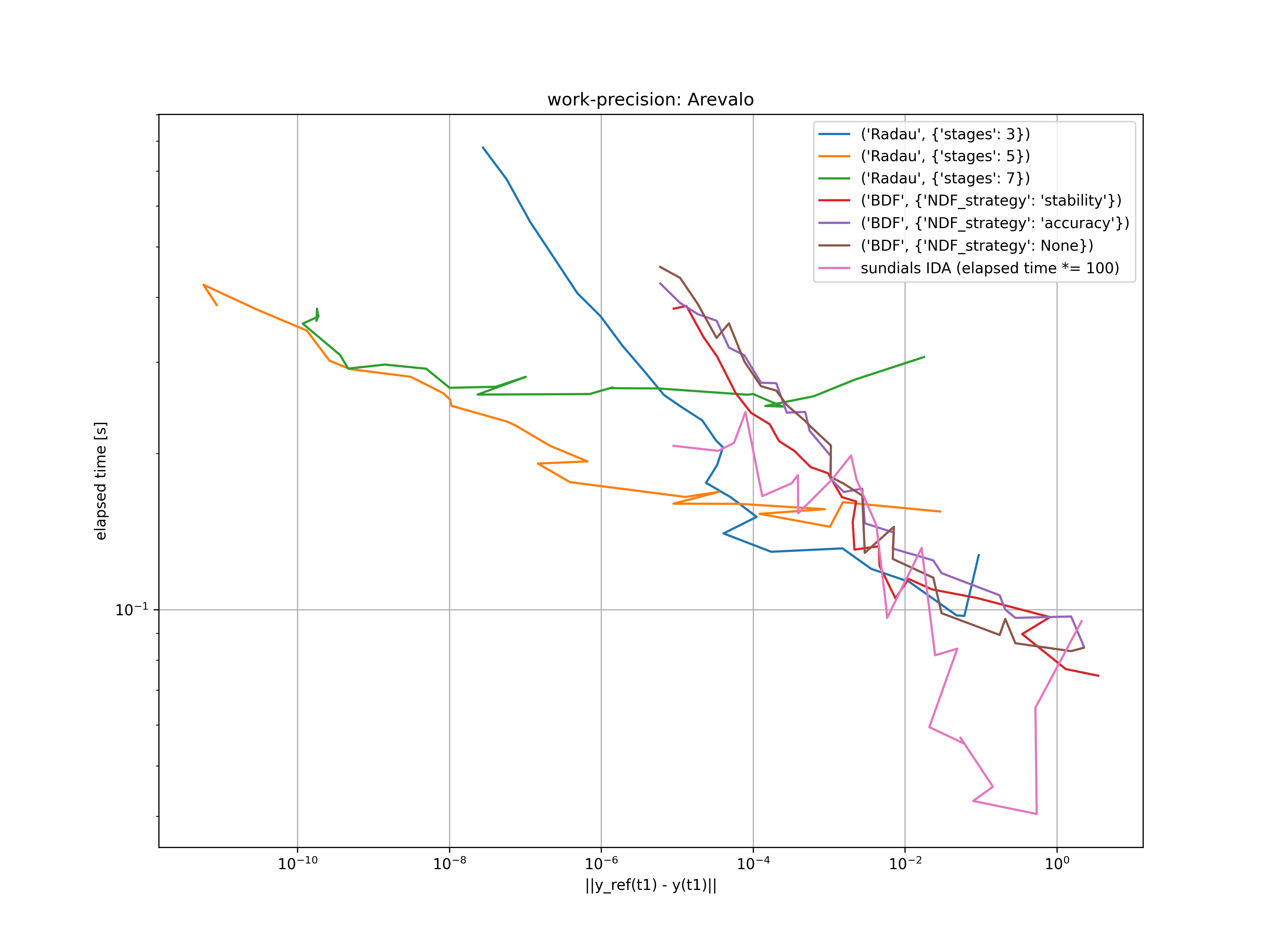
Index 3 DAE - Arevalo
Arevalo's index 3 problem describes the motion of a particle on a circular track. It is described by the system of differential algebraic equations
$$ \begin{aligned} \dot{x} &= u \ \dot{y} &= v \ \dot{u} &= 2 y + x \lambda \ \dot{v} &= -2 x + y \lambda \ 0 &= x^2 + y^2 - 1 . \end{aligned} $$
Since the implemented solvers are designed for index 1 DAEs we have to perform some sort of index reduction. Therefore, we use the stabilized index 1 formulation of Hiller and Anantharaman. The resulting index 1 system is given as
$$ \begin{aligned} \dot{x} &= u + x \dot{\Gamma} \ \dot{y} &= v + y \dot{\Gamma} \ \dot{u} &= 2 y + x \dot{\Lambda} \ \dot{v} &= -2 x + y \dot{\Lambda} \ 0 &= x u + y v \ 0 &= x^2 + y^2 - 1 . \end{aligned} $$
The analytical solution to this problem is given by
$$ \begin{aligned} x(t) &= \sin(t^2) \ y(t) &= \cos(t^2) \ u(t) &= 2 t \cos(t^2) \ v(t) &= -2 t \sin(t^2) \ \Lambda(t) &= -\frac{4}{3} t^3 \ \Gamma(t) &= 0 , \end{aligned} $$
with the Lagrange multipliers $\dot{\Lambda} = -4t^2$ and $\dot{\Gamma} = 0$.
This problem is solved for $atol = rtol = 10^{-(3 + m / 4)}$, where $m = 0, \dots, 24$. The resulting error at $t_1 = 5$ is compared with the elapsed time of the used solvers in the figure below.
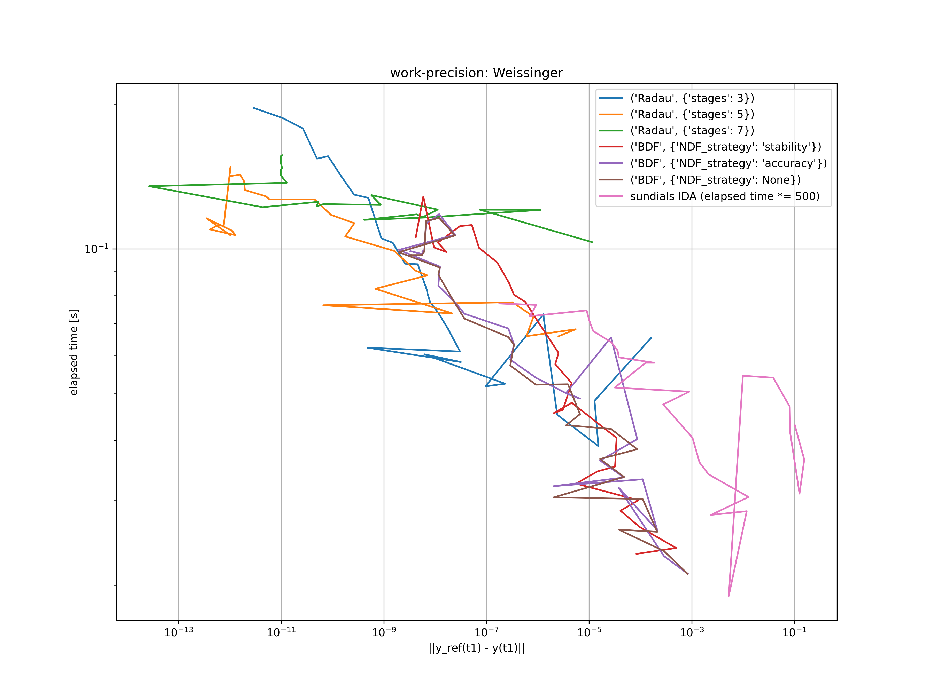
IDE - Weissinger
A simple example of an implicit differential equations is called Weissinger's equation
$$ t y^2 (\dot{y})^3 - y^3 (\dot{y}^2) + t (t^2 + 1) \dot{y} - t^2 y = 0 . $$
It has the analytical solution $y(t) = \sqrt{t^2 + \frac{1}{2}}$ and $\dot{y}(t) = \frac{t}{\sqrt{t^2 + \frac{1}{2}}}$.
Starting at $t_0 = \sqrt{1 / 2}$, this problem is solved for $atol = rtol = 10^{-(4 + m / 4)}$, where $m = 0, \dots, 28$. The resulting error at $t_1 = 10$ is compared with the elapsed time of the used solvers in the figure below.
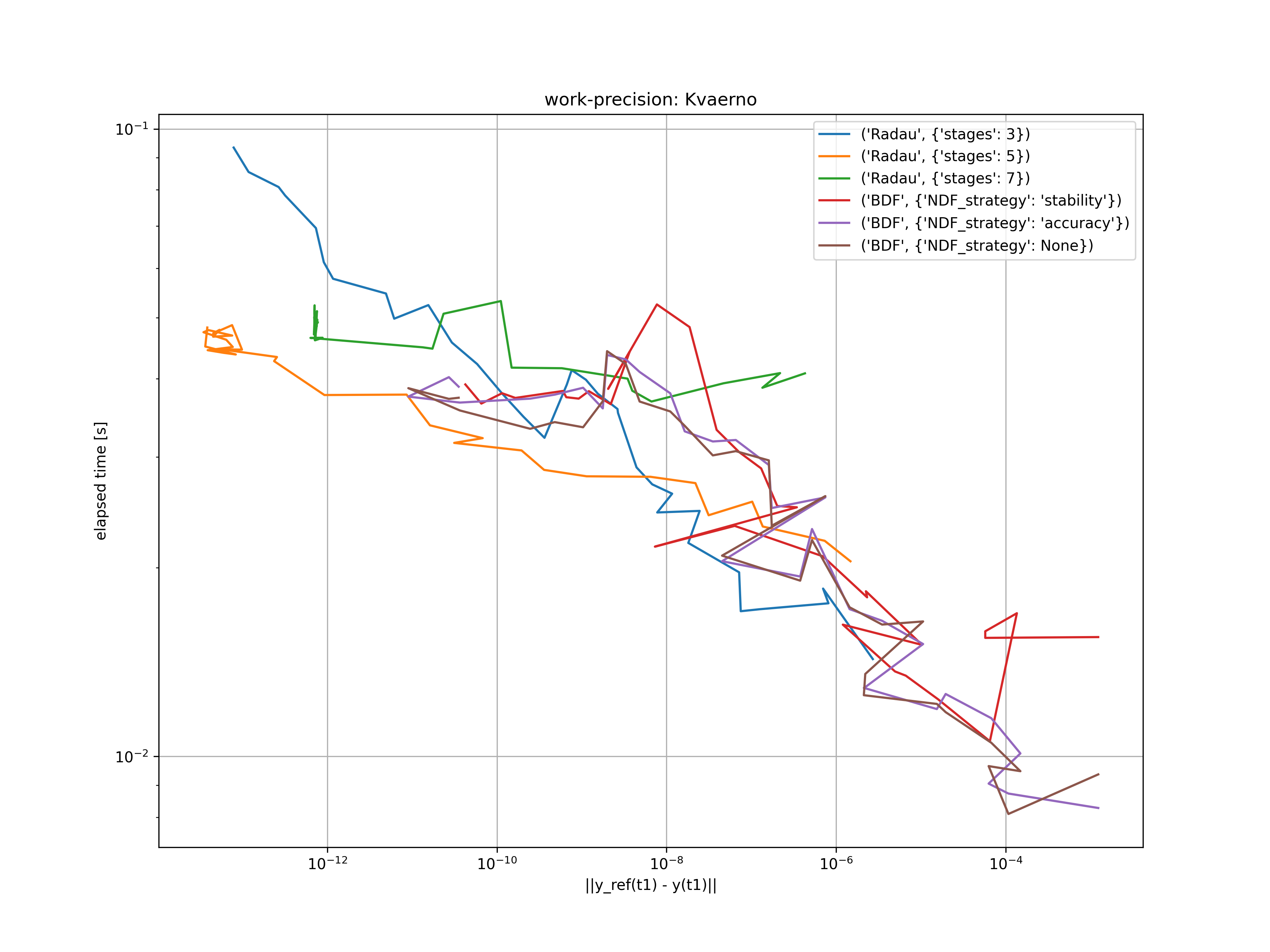
Nonlinear index 1 DAE - Kvaernø
In a final example, an nonlinear index 1 DAE is investigated as proposed by Kvaernø. The system is given by
$$ \begin{aligned} (\sin^2(\dot{y}_1) + \sin^2(y_2)) (\dot{y}_2)^2 - (t - 6)^2 (t - 2)^2 y_1 e^{-t} &= 0 \ (4 - t) (y_2 + y_1)^3 - 64 t^2 e^{-t} y_1 y_2 &= 0 , \end{aligned} $$
It has the analytical solution $y_1(t) = t^4 e^{-t}$, $y_2(t) = t^3 e^{-t} (4 - t)$ and $\dot{y}_1(t) = (4 t^3 - t^4) e^{-t}$, $y_2(t) = (-t^3 + (4 - t) 3 t^2 - (4 - t) t^3) e^{-t}$.
Starting at $t_0 = 0.5$, this problem is solved for $atol = rtol = 10^{-(4 + m / 4)}$, where $m = 0, \dots, 32$. The resulting error at $t_1 = 1$ is compared with the elapsed time of the used solvers in the figure below.
Install
Install through pip
To install solve-dae package you can run the command
pip install solve-dae
Install through git repository
To install the package through git installation you can download the repository and install it through
pip install .
Install for developing and testing
An editable developer mode can be installed via
python -m pip install -e .[dev]
The tests can be started using
python -m pytest --cov
Release history Release notifications | RSS feed


Download files
Download the file for your platform. If you're not sure which to choose, learn more about installing packages.
Source Distribution
Built Distribution
Filter files by name, interpreter, ABI, and platform.
If you're not sure about the file name format, learn more about wheel file names.
Copy a direct link to the current filters
File details
Details for the file solve_dae-0.2.3.tar.gz.
File metadata
- Download URL: solve_dae-0.2.3.tar.gz
- Upload date:
- Size: 70.8 MB
- Tags: Source
- Uploaded using Trusted Publishing? No
- Uploaded via: twine/6.2.0 CPython/3.12.3
File hashes
| Algorithm | Hash digest | |
|---|---|---|
| SHA256 |
0e31318521aef732afcd00fd722d02d6dde2a3ad5d3c9c2a1bb2001a247356cf
|
|
| MD5 |
be36fe0d2d3dd84cb538cefe9d17efd4
|
|
| BLAKE2b-256 |
563197f53d4eff48edd155276c394d11894eab8d030c9ea545cf2bbf0153234f
|
File details
Details for the file solve_dae-0.2.3-py3-none-any.whl.
File metadata
- Download URL: solve_dae-0.2.3-py3-none-any.whl
- Upload date:
- Size: 48.4 kB
- Tags: Python 3
- Uploaded using Trusted Publishing? No
- Uploaded via: twine/6.2.0 CPython/3.12.3
File hashes
| Algorithm | Hash digest | |
|---|---|---|
| SHA256 |
cccfc99980250dff317c0a7a67d386156cbdebe4bb34e863c0a6501542c46cff
|
|
| MD5 |
7145cfa1805a8192b59d3b8ed09cdf90
|
|
| BLAKE2b-256 |
51e3857143f2dcb4a3e69741c7f8bcd723c339afbeabd694d17265c25d55498f
|


